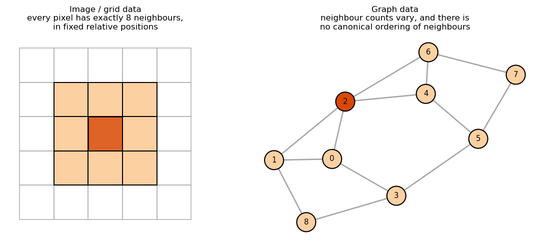
A neural network layer that operates on a graph has to combine information from a node’s neighbours.
The simplest way to do that is to average them. But should a node really listen to all of its neighbours equally?
Graph Attention Networks (GATs) say no, and let the model learn how much attention to pay to each neighbour.
Topics
Why graphs break ordinary neural networks, and the message-passing fix
The attention mechanism, built up one step at a time
A complete worked example with real numbers, from input all the way to the loss
Trade-offs, limitations, and a runnable PyTorch Geometric implementation
Recall the nomenclature
Definition. A graph \(G = (V, E)\) is a set of nodes (vertices) \(V\) and a set of edges\(E\) connecting pairs of them.
Notation we will use throughout
\(N = |V|\) is the number of nodes; nodes are indexed \(i, j\)
\(\mathcal{N}(i)\) is the neighbourhood of node \(i\): the set of nodes connected to \(i\) by an edge. By convention here it includes \(i\) itself (a “self-loop”).
\(d_i = |\mathcal{N}(i)|\) is the degree of node \(i\), i.e. how many neighbours it has
\(A \in \{0,1\}^{N \times N}\) is the adjacency matrix: \(A_{ij} = 1\) if there is an edge between \(i\) and \(j\)
Nodes carry data too
Every node \(i\) has a feature vector\(h_i \in \mathbb{R}^{F}\), where \(F\) is the number of features
Stacked together these form the feature matrix \(X \in \mathbb{R}^{N \times F}\)
Running example: a citation network
Nodes are academic papers, edges are citations
\(h_i\) is a bag-of-words vector describing the abstract of paper \(i\)
The label of a node is the paper’s subject area
Key point: a graph dataset gives you two independent sources of signal, the node features and the wiring. A good model uses both.
Learning Task: Node Classification
Setup
We are given one graph, the features \(X\) for every node, and the true labels \(y_i\) for only a small subset of nodes
Goal: predict the labels of the remaining nodes
This is called semi-supervised and transductive learning
Semi-supervised: most nodes are unlabelled, but their features and their edges still contribute to training
Transductive: the unlabelled test nodes are present in the graph during training. We are filling in holes, not generalising to a brand-new graph.
Concrete instance: the Cora dataset
\(2{,}708\) papers, \(10{,}556\) citation edges, \(7\) subject areas
\(F = 1{,}433\) binary bag-of-words features per paper
Only \(140\) labelled nodes for training, about \(5\%\) of the graph
The assumption that makes this possible: homophily
Connected nodes tend to share labels. Papers cite papers about the same topic.
Almost every standard GNN, GAT included, leans on this. Keep it in mind, we will return to it.
Recall: Message Passing
Nearly every modern graph neural network is one idea repeated: each node updates itself using a summary of its neighbours.
One layer, three steps
Message. Each neighbour \(j \in \mathcal{N}(i)\) produces a vector to send to \(i\).
Aggregate. Combine the incoming messages with a function that ignores their order, e.g. sum, mean, or max.
Update. Combine the aggregate with node \(i\)’s own current state to produce \(h_i'\).
Sum, mean, and max do not care how you list the neighbours, which is exactly the permutation symmetry we needed
They also accept any number of inputs, which handles variable degree
Different GNNs are just different choices of these three functions. GCN, GraphSAGE, GIN and GAT all fit this template. GAT’s contribution is entirely in the AGGREGATE step.
One Layer Equals One Hop
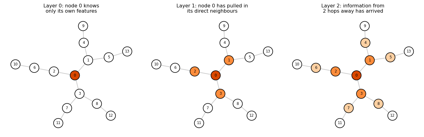
Each message-passing layer widens a node’s field of view by exactly one hop.
After \(L\) layers, node \(i\)’s representation depends on every node within distance \(L\) of \(i\)
This is the direct analogue of the growing receptive field in a deep CNN
Practical consequence
Two layers is the standard starting point, because most useful signal in a homophilous graph lives within two hops
Going deeper is surprisingly hard. With many layers, every node aggregates from nearly the whole graph and all the representations drift toward the same vector. This failure mode is called over-smoothing, and it is why GNNs are usually shallow while CNNs are deep.
Baseline comparison: The Graph Convolutional Network
The GCN layer (Kipf and Welling, 2017) is the simplest useful instance of the recipe. It is the model GAT was designed to improve on, so it is worth writing out.
\(W \in \mathbb{R}^{F' \times F}\) is a learned weight matrix, shared by every node, that maps features from dimension \(F\) to a new dimension \(F'\)
\(c_{ij}\) is a scalar mixing coefficient for the edge from \(j\) to \(i\)
\(\sigma\) is a nonlinearity such as ReLU
The self-loop means node \(i\) appears in its own sum, so it does not forget itself
Why normalise by \(\sqrt{d_i d_j}\)?
Without it, high-degree nodes accumulate huge sums and the scale of \(h_i'\) explodes
The symmetric \(1/\sqrt{d_i d_j}\) form also damps the influence of hub nodes that are connected to everything
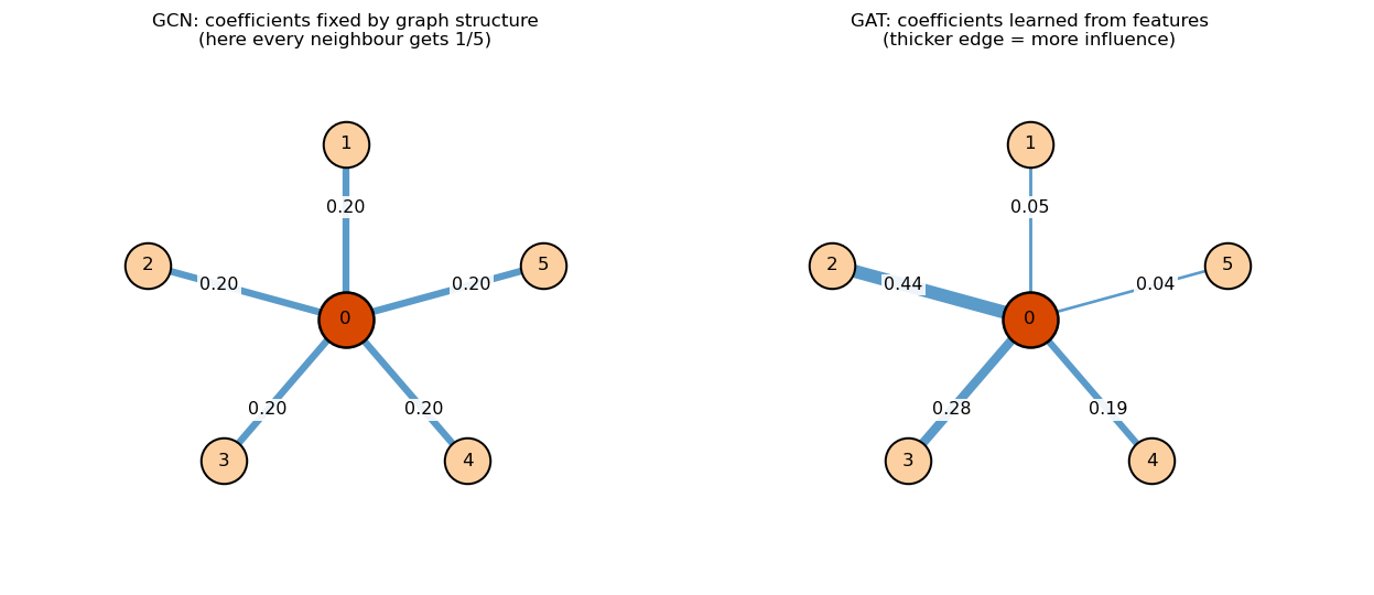
The essential observation:\(c_{ij}\) depends only on the degrees. It is fully determined by the graph’s wiring the moment you load the data, before a single gradient step.
The Limitation: Not All Neighbours Matter Equally
Example: Classifying a paper by its subject, it cites five others:
Two are directly relevant (very informative)
Two are generic methods cited by all fields
One is an irrelevant courtesy citation
GCN give every neighbour a weight based only on citation count, ignoring content. They can’t identify that the first two are truly useful—they never consult node features when weighting edges.
What’s wrong with \(c_{ij} = 1/\sqrt{d_i d_j}\)?
Structure-only: Neighbours with equal degrees get equal weights, even if their features differ greatly.
Not learned: Training doesn’t affect coefficients.
Graph-tied: Changing edges alters all neighbourhood weights.
Key question:
Can we make coefficients a learned function of both nodes’ features?
Use softmax to get normalized, positive weights: \(\alpha_j = \dfrac{\exp(e_j)}{\sum_k \exp(e_k)}\)
Output is the weighted sum: \(\sum_j \alpha_j v_j\)
Softmax recap: Transforms numbers into a probability distribution, exaggerating differences (e.g., scores \(2.5\) vs \(0.5\) become about \(7{:}1\) ratio) and making weights sum to \(1\).
Key points:
Weights are learned from context at each step (not fixed).
This is the mechanism powering Transformer models.
In a graph: The “query” is the current node; “keys” are its neighbours.
The GAT Layer
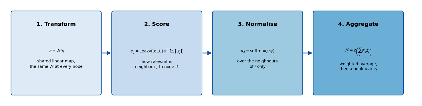
Everything that follows is an expansion of the four boxes below . The complete layer, written in one line, is
\[h_i' = \sigma\!\left( \sum_{j \in \mathcal{N}(i)} \alpha_{ij} \, W h_j \right)
\qquad\text{with}\qquad
\alpha_{ij} = \frac{\exp\!\left(\mathrm{LeakyReLU}\!\left(a^\top [W h_i \,\Vert\, W h_j]\right)\right)}
{\displaystyle\sum_{k \in \mathcal{N}(i)} \exp\!\left(\mathrm{LeakyReLU}\!\left(a^\top [W h_i \,\Vert\, W h_k]\right)\right)}\]
Symbols unpacked: - \([\,\cdot \,\Vert\, \cdot\,]\) means concatenation: \(z_i\) and \(z_j\) combined into length \(2F'\) - \(a \in \mathbb{R}^{2F'}\) is a learnable vector; \(a^\top[\cdot]\) is a single scalar - \(\mathrm{LeakyReLU}(x)\): \(x\) if \(x \ge 0\), \(0.2x\) otherwise: negative scores compressed, but not discarded
Simplification: split \(a\) into \(a = [a_{\text{src}} \,\Vert\, a_{\text{dst}}]\), get
So each node computes two scalars (\(a_{\text{src}}^\top z_i\), \(a_{\text{dst}}^\top z_j\)), and each edge score is their sum: making GAT efficient (how PyTorch Geometric implements it).
Key points: - \(e_{ij}\) is unnormalised; real-valued, positive or negative - \(e_{ij} \ne e_{ji}\), so attention is asymmetric (even if the graph is undirected) - \(e_{ij}\) is computed only for edges, not all \(N^2\) pairs
Read the subscript carefully. The sum in the denominator runs over \(k \in \mathcal{N}(i)\) only, the neighbours of \(i\). This is the masking, and it is where the graph structure enters the attention mechanism.
Why normalise at all?
Comparability. A node with 3 neighbours and a node with 300 now produce outputs on the same scale, which keeps training stable.
Interpretability. The coefficients form a probability distribution over neighbours: \(\alpha_{ij} \ge 0\) and \(\sum_j \alpha_{ij} = 1\). You can read them as “what fraction of its attention does node \(i\) spend on node \(j\)”.
Bounded output. The result is a convex combination of the \(z_j\), so \(h_i'\) can never blow up beyond the range of its inputs.
Two things students commonly get wrong
The softmax is taken per target node, one small softmax for each node’s own neighbour list, not one giant softmax over all edges
\(\alpha_{ij} \ne \alpha_{ji}\). Node \(i\) may spend most of its attention on \(j\) while \(j\) barely notices \(i\), because they have different neighbour sets to normalise against.
Take the transformed neighbour features, weight them by their attention, add them up
Pass the result through a nonlinearity \(\sigma\), usually \(\mathrm{ELU}\) in hidden layers
Reminder: ELU. The Exponential Linear Unit is \(\mathrm{ELU}(x) = x\) for \(x \ge 0\) and \(e^x - 1\) for \(x < 0\). Like ReLU on the positive side, but smooth and slightly negative rather than flat zero on the other, which keeps gradients alive.
The role of the self-loop, one more time
Because \(i \in \mathcal{N}(i)\), the sum includes the term \(\alpha_{ii} z_i\). Without it, a node’s new representation would be built entirely out of its neighbours and would discard its own features. Every practical implementation adds self-loops before the first layer.
Sanity checks worth internalising
The weights sum to one, so \(h_i'\) is an average, not a sum. Doubling a node’s degree does not double the magnitude of its output.
Output dimension is \(F'\), set by the shape of \(W\), and has nothing to do with the node’s degree
If you froze all \(\alpha_{ij}\) at \(1/d_i\), you would recover mean-aggregation, i.e. essentially a GCN
Multi-Head Attention
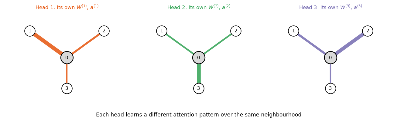
One attention pattern is a single point of view. In practice GAT runs \(K\) independent attention mechanisms, called heads, in parallel.
Each head \(k\) has its own parameters\(W^{(k)}\) and \(a^{(k)}\), and produces its own output \(h_i'^{(k)} \in \mathbb{R}^{F'}\).
Stability. Averaging several independently initialised attention patterns smooths out a noisy single one, much as an ensemble does.
Diversity. Different heads can specialise. One may track topical similarity, another may focus on highly cited hubs.
Capacity. It is the graph analogue of using many filters in a CNN layer rather than one.
Dimension bookkeeping, which trips people up. With \(F' = 8\) and \(K = 8\) heads and concatenation, the layer outputs \(8 \times 8 = 64\) features per node. The next layer must therefore expect an input of size \(64\), not \(8\).
Putting a Full Network Together
A standard two-layer GAT for node classification on Cora
Input:\(X \in \mathbb{R}^{2708 \times 1433}\), plus the edge list
Dropout on the input features, \(p = 0.6\)
GAT layer 1:\(F' = 8\), \(K = 8\) heads, concatenated, ELU activation \(\Rightarrow\) output is \(2708 \times 64\)
Dropout again, \(p = 0.6\)
GAT layer 2:\(F' = 7\) (one per class), \(K = 1\) head \(\Rightarrow\) output is \(2708 \times 7\)logits
Loss: softmax cross-entropy, computed only on the labelled training nodes
Reminder: logits. The raw, unnormalised scores that come out of the final layer, one per class. Applying a softmax to logits gives predicted class probabilities. In PyTorch you almost always feed logits directly into CrossEntropyLoss, which applies the softmax internally for numerical stability.
Dropout in a GAT deserves special mention
Standard dropout randomly zeroes input features
GAT additionally applies dropout to the attention coefficients themselves, which randomly disconnects edges during training
With only 140 labelled nodes, this aggressive regularisation is doing a lot of work
A Worked Example, Start to Finish
The Setup
We will push node 1 through a complete single-head GAT layer and out to a loss value, doing every arithmetic step explicitly.
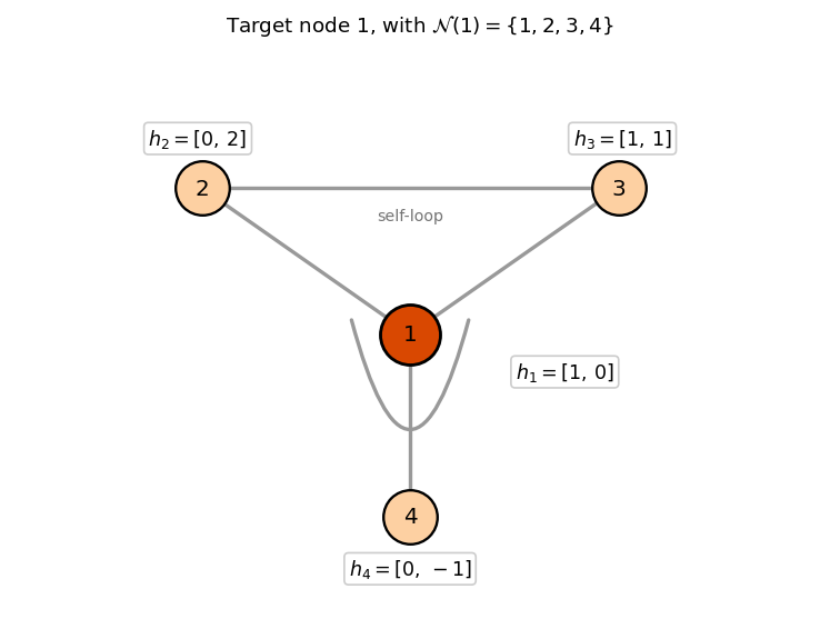
The graph. Four nodes. Node 1 is connected to nodes 2, 3 and 4, and to itself. So \(\mathcal{N}(1) = \{1, 2, 3, 4\}\).
Note what this step is and is not. It is applied to each node completely independently. No information has crossed any edge yet. This is just a dense layer.
Step 2: Score Each Neighbour
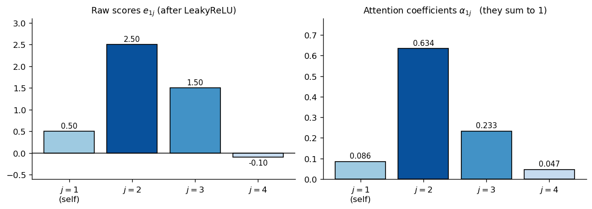
Use the split form \(e_{1j} = \mathrm{LeakyReLU}\left(a_{\text{src}}^\top z_1 + a_{\text{dst}}^\top z_j\right)\).
The source term is computed once and reused for all four edges
Node 1 spends about \(63\%\) of its attention on node 2, and under \(5\%\) on node 4
A GCN on this same neighbourhood would have handed out fixed coefficients based purely on degree, ignoring the fact that node 2’s features are the informative ones
Notice how much the exponential exaggerates: a score gap of \(2.5 - 1.5 = 1\) became a weight ratio of roughly \(2.7{:}1\)
Sanity check on the result. Every \(z_j\) had components in \([-2, 4]\), and the output components sit comfortably inside that range. Because the \(\alpha\) values are non-negative and sum to one, this is guaranteed: the output is always inside the convex hull of the transformed neighbour features.
Cross-entropy loss. For a single example with true class \(c\), the loss is \(\mathcal{L} = -\log \hat{p}_c\). The true label is class 0, so
\[\mathcal{L} = -\log(0.094) = 2.368\]
Read what just happened. The model predicts class 1 with \(90.6\%\) confidence, and it is wrong. That is a large loss, exactly as it should be for an untrained network. The next step is backpropagation.
What Gradient Descent Actually Changes
Backpropagation computes \(\partial \mathcal{L} / \partial \theta\) for every parameter and nudges each one downhill. In our layer that means three things:
\(W_{\text{out}}\), the classifier
\(W\), the shared feature transform
\(a\), the attention vector
The third one is the interesting one. Because \(\alpha_{1j}\) is a differentiable function of \(a\), the gradient flows all the way into the attention mechanism. Training does not just adjust what each node’s features become; it adjusts which neighbours each node listens to.
If down-weighting node 4 and up-weighting node 2 would have reduced the loss, the gradient step moves \(a\) in a direction that does exactly that, for every node in the graph at once, since \(a\) is shared.
Contrast with the GCN. There, the coefficient \(1/\sqrt{d_i d_j}\) is a constant. It has no gradient. It is the same on the first epoch and the last. This one difference is the entire contribution of the paper.
A caveat worth stating. Attention is not magic. It adds a modest number of parameters and a modest amount of flexibility. On graphs where all neighbours genuinely are equally informative, a GCN can match or beat a GAT.
Properties, Trade-offs, and Practice
GAT versus GCN at a Glance
GCN
GAT
Neighbour weight
\(1/\sqrt{d_i d_j}\), fixed
\(\alpha_{ij}\), learned from features
Uses node features to weight edges
no
yes
Symmetric weights
yes
no, \(\alpha_{ij} \ne \alpha_{ji}\)
Extra parameters per layer
none
\(a \in \mathbb{R}^{2F'}\) per head
Cost
\(O(\lvert E \rvert F')\)
\(O(\lvert E \rvert F')\), same order
Needs the whole graph at once
in the classic formulation, yes
no
Handles unseen nodes and graphs
awkwardly
naturally
Gives edge-level scores you can inspect
no
yes
Two rows deserve elaboration
Unseen nodes. GAT’s parameters \(W\) and \(a\) are functions of features only, never of node identity or of a fixed graph-wide normalisation. Train on one protein interaction network, run on a different one. This makes GAT genuinely inductive.
Same order of cost. Both scale linearly in the number of edges. Attention is not the expensive part of a GNN; the feature transform is.
Cost and Scalability
Time complexity of a single GAT head
\[O\big(\underbrace{N F F'}_{\text{the } W h_i \text{ transforms}} + \underbrace{\lvert E \rvert F'}_{\text{the edge scores and aggregation}}\big)\]
Linear in the number of edges, which is the key property. Real graphs are sparse, so \(\lvert E \rvert \ll N^2\).
With \(K\) heads, multiply by \(K\). Heads are fully parallel, so on a GPU this is nearly free.
What GAT deliberately avoids
No matrix inversion, no eigendecomposition of the Laplacian, unlike earlier spectral graph convolution methods
No requirement to know the full graph structure up front, unlike the classic GCN normalisation
Where it does get hard
Memory is \(O(\lvert E \rvert)\) per head for storing the attention coefficients. On a graph with a hundred million edges this bites.
The standard fix is neighbour sampling: for each target node, sample a fixed number of neighbours per layer and build mini-batches from those subgraphs. In PyTorch Geometric this is NeighborLoader.
On Interpreting Attention Weights
It’s tempting to plot learned \(\alpha_{ij}\) and conclude which edges matter—proceed with caution.
Fair interpretations - \(\alpha_{ij}\) indicates the proportion of transformed features from neighbor \(j\) to node \(i\) in a specific head/layer. - Comparing attention patterns between models (trained vs. untrained) can highlight useful differences. - Helpful for generating hypotheses to explore further.
Misinterpretations to avoid - “High attention = importance”: Large \(\alpha_{ij}\) doesn’t guarantee significant influence—neighbor features could be negligible. - “This explains the model”: Multiple heads and layers mean many, often inconsistent, attention maps. - “It’s stable”: Changing the random seed can alter attention patterns with no change in accuracy.
Key takeaway: Like Transformer attention in NLP, GAT attention is evidence, not explanation. For true attribution, use tools like GNNExplainer.
Look at what depends on what. The term involving the neighbour \(j\) is \(a_{\text{dst}}^\top z_j\), and it does not involve \(i\) at all. The query node contributes only an additive constant, exactly as we saw in the worked example where \(a_{\text{src}}^\top z_1 = 0.5\) appeared in all four rows.
The consequence. Since LeakyReLU is monotonic, adding the same constant to every score cannot change their ranking. So the ordering of neighbours by attention is the same for every query node in the graph. Some node is globally the most attractive neighbour, and every node that touches it ranks it first. This is called static attention.
GATv2 fixes it (Brody, Alon and Yahav, 2022) by moving the nonlinearity inside, before the dot product with \(a\):
Now \(z_i\) and \(z_j\) interact through the nonlinearity before \(a\) sees them, so the ranking genuinely depends on the query. This is dynamic attention, and it is strictly more expressive.
Practically: in PyTorch Geometric, swap GATConv for GATv2Conv. Same interface, usually equal or better results, marginally more compute. For new projects it is a reasonable default.
Practical Tips and Common Pitfalls
Things to do
Add self-loops.GATConv does this by default. Without them nodes discard their own features.
Normalise your features. Row-normalising bag-of-words features is standard and matters on Cora.
Use dropout on the attention coefficients, not just the inputs. On small labelled sets, \(p = 0.6\) is a common and surprisingly aggressive choice.
Start with 2 layers, 8 hidden units, 8 heads. These are the paper’s settings and they are a sane baseline.
Track a validation set and stop early. These models overfit 140 labels very quickly.
Things to watch out for
Dimension mismatch between layers. With concatenation, layer 2’s input size is \(K \times F'\), not \(F'\). This is the single most common bug.
Over-smoothing. Piling on layers usually makes things worse, not better. If you need depth, add residual connections.
Heterophilous graphs. If connected nodes tend to have different labels, as in some fraud or dating networks, the whole “aggregate your neighbours” premise is shaky. Attention helps somewhat, since it can learn to down-weight, but it cannot produce negative weights, so it can never actively contrast against a neighbour. Specialised architectures exist for this setting.
Do not assume GAT beats GCN. On several standard benchmarks the gap is within noise. Measure it.
Code Demo:
A Hello-World GAT
Statement of problem
We will train a two-layer GAT to classify papers in the Cora citation network, using PyTorch Geometric, the standard library for graph deep learning in PyTorch.
Why this counts as a real starting point, not a toy
All hyperparameters live in a single dictionary, so the whole thing drops straight into Optuna, Ray Tune, or a plain grid search
The model is a proper nn.Module with a clean forward, so it composes with anything else in PyTorch
Training and evaluation are separate functions with correct train() / eval() mode handling and no_grad() on evaluation
We track validation accuracy and keep the best checkpoint, rather than reporting whatever the last epoch happened to produce
Requirements
pip install torch torch_geometric
Cora downloads automatically the first time you run it, and is only a few megabytes. Everything here runs comfortably on a CPU in well under a minute.
Code
import torchimport torch.nn as nnimport torch.nn.functional as Fimport torch_geometric.transforms as Tfrom torch_geometric.datasets import Planetoidfrom torch_geometric.nn import GATConvtorch.manual_seed(42)DEVICE = torch.device("cuda"if torch.cuda.is_available() else"cpu")# NormalizeFeatures row-normalises the bag-of-words vectors, which is the# standard preprocessing step for the Planetoid citation datasets.dataset = Planetoid(root="data/Planetoid", name="Cora", transform=T.NormalizeFeatures())data = dataset[0].to(DEVICE)print(f"Nodes: {data.num_nodes}")print(f"Edges: {data.num_edges}")print(f"Features/node: {dataset.num_features}")print(f"Classes: {dataset.num_classes}")print(f"Training nodes: {int(data.train_mask.sum())}")print(f"Validation nodes: {int(data.val_mask.sum())}")print(f"Test nodes: {int(data.test_mask.sum())}")
Nodes:            2708
Edges:            10556
Features/node:    1433
Classes:          7
Training nodes:   140
Validation nodes: 500
Test nodes:       1000
Understanding the Data Object
A PyG Data object holds the whole graph in a few tensors.
data.x has shape [num_nodes, num_features], the feature matrix \(X\)
data.edge_index has shape [2, num_edges] and is the graph itself in COO format: column \(k\) is the pair [source, target] for the \(k\)-th directed edge. An undirected edge appears twice, once in each direction. This sparse edge list is why the memory cost is \(O(\lvert E \rvert)\) rather than \(O(N^2)\).
data.y has shape [num_nodes], the integer class label of every node
data.train_mask, val_mask, test_mask are boolean vectors of length num_nodes marking which nodes belong to which split
How the masks work, and why this is not like ordinary supervised learning
The forward pass runs over the entire graph every single time, computing a prediction for all 2,708 nodes. The masks are applied only when computing the loss and the metrics. Test nodes therefore participate in message passing during training, they just never contribute a label. That is what “transductive” means in practice.
Code
# All tunable knobs in one place, so this config can be swapped out by a# hyperparameter search without touching any of the code below.CONFIG = {# architecture"hidden_channels": 8, # F' per head in layer 1"heads": 8, # number of attention heads in layer 1"out_heads": 1, # heads in the output layer (averaged, not concatenated)"dropout": 0.6, # applied to inputs AND attention coefficients"negative_slope": 0.2, # the LeakyReLU slope inside the attention scores# optimisation"lr": 0.005,"weight_decay": 5e-4, # L2 regularisation, important with 140 labels"epochs": 200,"patience": 30, # early stopping patience, in epochs}for k, v in CONFIG.items():print(f"{k:>18}: {v}")
Two GATConv layers, with the dimension bookkeeping made explicit.
Trace the shapes for Cora
Input: [2708, 1433]
After layer 1 with heads=8 and hidden_channels=8, concatenated: [2708, 64]
After layer 2 with out_heads=1 and out_channels=7: [2708, 7] logits
Note the hidden_channels * heads in the second layer’s input size. That is the concatenation bookkeeping from earlier, and getting it wrong is the classic beginner error.
Two details in the code below
concat=False on the output layer makes it average the heads rather than concatenate them, matching the paper
We return raw logits, not probabilities. F.cross_entropy applies the log-softmax internally, which is both more numerically stable and less code.
Code
class GAT(nn.Module):"""A two-layer Graph Attention Network for node classification."""def__init__(self, in_channels, out_channels, cfg):super().__init__()self.dropout = cfg["dropout"]self.conv1 = GATConv( in_channels=in_channels, out_channels=cfg["hidden_channels"], heads=cfg["heads"], concat=True, # -> hidden_channels * heads negative_slope=cfg["negative_slope"], dropout=cfg["dropout"], # dropout on the attention coefficients )self.conv2 = GATConv( in_channels=cfg["hidden_channels"] * cfg["heads"], out_channels=out_channels, heads=cfg["out_heads"], concat=False, # average the heads instead negative_slope=cfg["negative_slope"], dropout=cfg["dropout"], )def forward(self, x, edge_index): x = F.dropout(x, p=self.dropout, training=self.training) x =self.conv1(x, edge_index) x = F.elu(x) x = F.dropout(x, p=self.dropout, training=self.training) x =self.conv2(x, edge_index)return x # raw logits, shape [N, num_classes]model = GAT(dataset.num_features, dataset.num_classes, CONFIG).to(DEVICE)optimizer = torch.optim.Adam(model.parameters(), lr=CONFIG["lr"], weight_decay=CONFIG["weight_decay"])n_params =sum(p.numel() for p in model.parameters() if p.requires_grad)print(model)print(f"\nTrainable parameters: {n_params:,}")
def train_one_epoch(model, data, optimizer):"""One full-batch gradient step. Loss is computed on training nodes only.""" model.train() optimizer.zero_grad() logits = model(data.x, data.edge_index) loss = F.cross_entropy(logits[data.train_mask], data.y[data.train_mask]) loss.backward() optimizer.step()returnfloat(loss)@torch.no_grad()def evaluate(model, data):"""Accuracy on each split. No gradients, dropout disabled.""" model.eval() logits = model(data.x, data.edge_index) preds = logits.argmax(dim=1) accs = {}for split in ["train", "val", "test"]: mask = data[f"{split}_mask"] accs[split] =float((preds[mask] == data.y[mask]).float().mean()) val_loss =float(F.cross_entropy(logits[data.val_mask], data.y[data.val_mask]))return accs, val_loss
Code
import copyhistory = {"epoch": [], "train_loss": [], "val_loss": [], "val_acc": []}best_val_acc, best_state, epochs_without_improvement =0.0, None, 0for epoch inrange(1, CONFIG["epochs"] +1): train_loss = train_one_epoch(model, data, optimizer) accs, val_loss = evaluate(model, data) history["epoch"].append(epoch) history["train_loss"].append(train_loss) history["val_loss"].append(val_loss) history["val_acc"].append(accs["val"])if accs["val"] > best_val_acc: best_val_acc = accs["val"] best_state = copy.deepcopy(model.state_dict()) epochs_without_improvement =0else: epochs_without_improvement +=1if epoch %25==0:print(f"epoch {epoch:3d} | train loss {train_loss:.4f} "f"| val loss {val_loss:.4f} | val acc {accs['val']:.4f}")if epochs_without_improvement >= CONFIG["patience"]:print(f"early stopping at epoch {epoch}")break# Always report the best checkpoint, never the last one.model.load_state_dict(best_state)final_accs, _ = evaluate(model, data)print(f"\nbest val accuracy : {best_val_acc:.4f}")print(f"test accuracy : {final_accs['test']:.4f}")
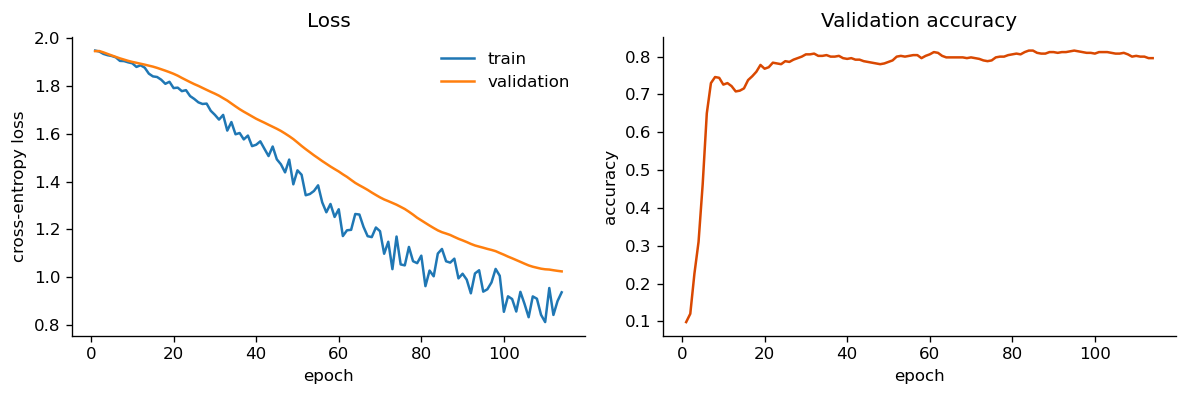
epoch  25 | train loss 1.7454 | val loss 1.8074 | val acc 0.7880
epoch  50 | train loss 1.4468 | val loss 1.5634 | val acc 0.7860
epoch  75 | train loss 1.0534 | val loss 1.2942 | val acc 0.7900
epoch 100 | train loss 0.8553 | val loss 1.0940 | val acc 0.8080
early stopping at epoch 114

best val accuracy : 0.8160
test accuracy     : 0.8240
Code
import matplotlib.pyplot as pltfig, axes = plt.subplots(1, 2, figsize=(10, 3.4))axes[0].plot(history["epoch"], history["train_loss"], label="train")axes[0].plot(history["epoch"], history["val_loss"], label="validation")axes[0].set_xlabel("epoch")axes[0].set_ylabel("cross-entropy loss")axes[0].set_title("Loss")axes[0].legend(frameon=False)axes[1].plot(history["epoch"], history["val_acc"], color="#d94801")axes[1].set_xlabel("epoch")axes[1].set_ylabel("accuracy")axes[1].set_title("Validation accuracy")for a in axes: a.spines[["top", "right"]].set_visible(False)plt.tight_layout()plt.show()
Reading the Training Curves
What you should expect to see
Test accuracy in the neighbourhood of \(0.80\) to \(0.83\), which is in line with the published result for GAT on Cora
Training loss falling much faster than validation loss, the signature of a model with far more capacity than it has labels
A validation accuracy curve that climbs quickly, then flattens and wobbles
Why the heavy regularisation is not optional here
With 1,433 input features and only 140 labelled nodes, the model could memorise the training set almost immediately. Three mechanisms hold it back: dropout at \(p = 0.6\) on both features and attention, weight decay of \(5\times 10^{-4}\), and early stopping on validation accuracy. Turn any one of them off and the test accuracy drops noticeably. This is a good experiment to run yourself.
A useful baseline for comparison. An MLP that ignores the graph entirely and classifies each paper from its own features alone reaches roughly \(0.55\) to \(0.60\) on Cora. The jump to \(0.80\) is what the graph structure buys you.
Code
# GATConv can hand back the attention coefficients it computed.# The returned edge_index includes the self-loops the layer adds internally.model.eval()with torch.no_grad(): _, (att_edge_index, att_weights) = model.conv1( data.x, data.edge_index, return_attention_weights=True )print(f"attention tensor shape: {tuple(att_weights.shape)} "f"# (edges including self-loops, heads)")# Inspect one node's neighbourhood, averaged over the eight heads.# Row 0 of edge_index is the source, row 1 is the target, and messages# flow source -> target, so we want the edges whose target is our node.target =0mask = att_edge_index[1] == targetsources = att_edge_index[0][mask].tolist()alphas = att_weights[mask].mean(dim=1).tolist()print(f"\nAttention paid by node {target} to its neighbours, "f"averaged over {CONFIG['heads']} heads:")for src, a insorted(zip(sources, alphas), key=lambda t: -t[1]): tag =" <- self-loop"if src == target else""print(f" alpha[{target} <- {src:4d}] = {a:.4f}{tag}")print(f"\nThese sum to {sum(alphas):.4f}, as the softmax guarantees.")
attention tensor shape: (13264, 8)   # (edges including self-loops, heads)

Attention paid by node 0 to its neighbours, averaged over 8 heads:
  alpha[0 <-    0] = 0.2530   <- self-loop
  alpha[0 <- 1862] = 0.2495
  alpha[0 <- 2582] = 0.2490
  alpha[0 <-  633] = 0.2485

These sum to 1.0000, as the softmax guarantees.
What to Try Next
Replace GATConv with GATv2Conv. The import and the constructor arguments are identical, and you get dynamic attention for free.
Set heads=1 and see how much the multi-head averaging was contributing.
Set dropout=0.0 and watch the test accuracy fall while the training loss goes to nearly zero.
Add a third layer and observe over-smoothing degrade the result rather than improve it.
Larger extensions
Hyperparameter search.CONFIG is already a plain dictionary; wrap the training loop in a function that takes it as an argument and hand it to Optuna.
Different datasets.Planetoid also provides CiteSeer and PubMed with a one-word change. For a heterophilous stress test, try the WebKB datasets, where GAT’s assumptions break down.
Scale up. Swap full-batch training for NeighborLoader to handle graphs that do not fit in memory.
Different tasks. The same encoder works for graph classification (add a global pooling layer) and link prediction (score node pairs by a dot product of their embeddings).
Edge features.GATConv accepts an edge_dim argument, letting edge attributes enter the attention score.