Timeline of the GNN Architecture Landscape
The Landscape at a Glance
Prehistory: before the 2014 deep learning rebirth (1997–2009)
- Recursive Neural Networks (1997, Sperduti & Starita): First neural method for structured data (trees); limited to acyclic structures.
- Graph Neural Network Model (2005/2009, Gori, Monfardini & Scarselli): Named the field; introduced iterative node updates to fixed point, but theory and hardware were not ready.
Shallow embeddings: a detour (2014–2016)
- DeepWalk (2014, Perozzi et al.): Used random walks + word2vec to encode graph structure; ignored node features and could not generalize to new nodes (i.e. transductive).
- node2vec (2016, Grover & Leskovec): Improved DeepWalk by tuning walks for roles vs. communities; still transductive and feature-agnostic.
The spectral route: convolution foundations (2014–2017)
- Spectral CNN (2014, Bruna et al. and Yann LeCun): Defined spectral convolution via Laplacian eigenbasis; mathematically elegant but computationally impractical and not transferable.
- ChebNet (2016, Defferrard et al.): Approximated filters with Laplacian polynomials; efficient, local, and transferable across graphs.
- GCN (2017, Kipf & Welling): Simplified ChebNet to \(K{=}1\); average neighbors then transform: practical breakthrough, mainstreamed spatial models.
Message-passing era: unified language (2017–2018)
- GraphSAGE (2017, Hamilton, Ying & Leskovec): Inductive; samples neighbors for scalable minibatching, flexible aggregation.
- GAT (2018, Veličković et al.): Introduced attention for learnable edge weights; more robust to noise.
- MPNN (2017, Gilmer et al.): Defined all these as message→aggregate→update; unified framework, not a model.
Theory: limits of message passing (2018–2021)
- GIN / WL ceiling (2019, Xu et al.): Matched 1-WL test in graph discrimination; showed sum > mean/max aggregation.
- Oversmoothing (2018, Li et al.): Stacking layers causes all node vectors to converge; restricts depth.
- Oversquashing (2021, Alon & Yahav): Bottleneck: too many nodes’ info crammed into fixed-size reps; long-range dependencies lost.
Geometric / equivariant GNNs (2017–present)
- SchNet (2017, Schütt et al.): Learned on interatomic distances; ensures rotation invariance but can’t capture angles.
- DimeNet (2020, Gasteiger et al.): Adds angle information via edge-level messaging.
- Tensor Field Networks / SE(3)-Transformer (2018/2020): Fully equivariant to rotations; mathematically exact.
- NequIP (2021, Batzner et al.): Highly data-efficient equivariant models for atomic potentials.
- MACE (2022, Batatia et al.): Built high-order interactions in a single layer; faster, more stable.
- MACE-MP / GNoME and successors (2023–2026): Pretrained universal interatomic models; efficient fine-tuning for DFT accuracy.
Graph transformers: global mechanisms (2020–2023)
- Graphormer (2021, Microsoft Research): Structural biases built into transformer; state-of-the-art on benchmarks.
- GraphGPS (2022, Rampášek et al.): Merged local message passing + global attention per layer; practical for small/medium graphs.
- Limitation: Attention is \(O(n^2)\): great for molecules, impractical for very large graphs.
Motivation and Terminology
Why Graphs Are Hard
- Deep learning first mastered images and sequences, not because they’re most important, but because both have a clear grid.
- Convolutions slide a small set of weights over the input, relying on “one position to the right” meaning the same thing everywhere.
- Weight sharing—using the same filter everywhere—makes CNNs efficient (9 numbers process a 10-megapixel image) and generalizable (learn an edge detector once and apply it everywhere).
- Graphs (molecules, social networks, citation graphs, etc.) have no grid: One node may have 3 neighbors, another 11,000. There’s no “up,” and no fixed neighbor ordering.
Vocabulary.
- Graph \(G = (V, E)\): nodes (vertices) and edges (relationships).
- Degree \(d_i\): how many edges touch node \(i\).
- Neighborhood \(\mathcal{N}(i)\): the set of nodes adjacent to \(i\).
- Adjacency matrix \(A \in \{0,1\}^{n \times n}\): \(A_{ij} = 1\) if there is an edge \(i \to j\).
- Node feature matrix \(X \in \mathbb{R}^{n \times d}\): one row per node.
The Core Problem Is Symmetry
Relabel the nodes and you get a completely different matrix describing an identical object.
\[A \;\longmapsto\; P A P^{\top}, \qquad X \;\longmapsto\; P X\]
where \(P\) is a permutation matrix. There are \(n!\) such relabelings.
Two words we will use constantly:
- Invariant: the transformation does not change the output: \(f(PAP^\top, PX) = f(A, X)\).
- Example: shift an image ten pixels right; “this is a cat” is unchanged.
- Graph example: predicting whether a molecule is toxic.
- Equivariant: the output transforms the same way the input did: \(f(PAP^\top, PX) = P\,f(A, X)\).
- Example: shift an image ten pixels right; the segmentation mask shifts ten pixels right.
- Graph example: predicting a label for every node.
Key idea: thirty years of GNN research is one sustained attempt to answer “how do we build a network whose architecture respects the symmetry of the domain?”: and later, “what if the domain also has geometric symmetries like rotations and translations in molecules?”
Jargon and nomenclature
| Term | Meaning |
|---|---|
| Adjacency matrix \(A\) | \(n \times n\) table of which nodes connect |
| Laplacian \(L=D-A\) | discrete second derivative; measures roughness |
| Aggregation | permutation-invariant combination of neighbor messages |
| Invariant / equivariant | output unchanged / output transforms with the input |
| Transductive / inductive | answers only for seen items / a general reusable function |
| Multiset | a set that records how many times each element appears |
| Receptive field | region of input an output depends on; \(L\) hops after \(L\) layers |
| Oversmoothing | representations converge to identical values with depth |
| Oversquashing | exponentially many nodes squeezed into one fixed-size vector |
| WL test | color-refinement heuristic; the expressivity ceiling for message passing |
| Body order | how many atoms one interaction term involves at once |
| Readout / pooling | collapsing node representations into one graph-level vector |
Recall: The Graph Laplacian
The Laplacian measures how much a function at a point differs from the average nearby: a discrete second derivative.
\[L = D - A, \qquad D = \mathrm{diag}(d_1, \ldots, d_n)\]
Applied to a signal \(x\) on the nodes:
\[(Lx)_i = d_i x_i - \sum_{j \in \mathcal{N}(i)} x_j = \sum_{j \in \mathcal{N}(i)} (x_i - x_j)\]
- Each entry is the total disagreement between node \(i\) and its neighbors. \(L\) measures roughness.
- The quadratic form makes this explicit: \(\;x^\top L x = \sum_{(i,j) \in E} (x_i - x_j)^2 \geq 0\).
- Eigenvectors of \(L\) = the graph’s natural “frequencies.”
- Small eigenvalue \(\Rightarrow\) eigenvector varies smoothly across the graph.
- Large eigenvalue \(\Rightarrow\) eigenvector flips sign between neighbors.
Normalized version (keeps eigenvalues in a small range, which matters for stacking layers):
\[L_{\text{sym}} = I - D^{-1/2} A D^{-1/2}\]
Spectral methods and GCNs
Spectral Convolution on Graphs
Spectral graph neural networks transform a graph into a spectrum of “frequencies”, measuring how features vary across nodes, so the model can amplify key structural patterns and then project the filtered result back onto the nodes.
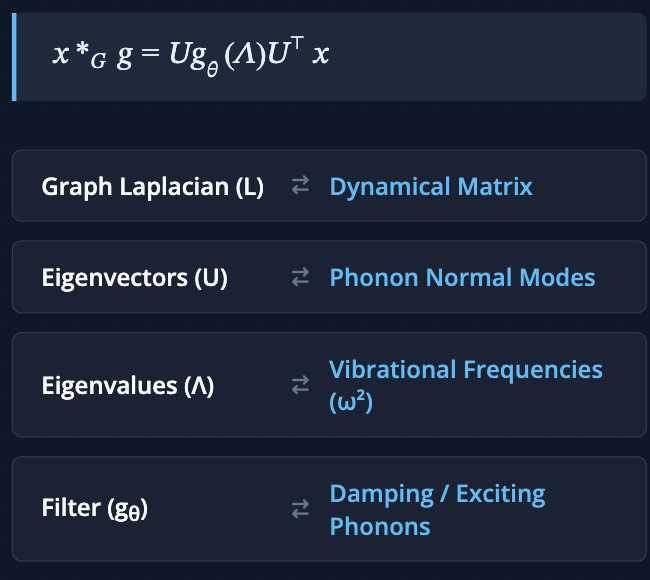
Bruna et al. (2014) applied the convolution theorem to graphs: spatial convolution equals pointwise frequency multiplication. By diagonalizing the Graph Laplacian (\(L=U \Lambda U^{\top}\)), spectral convolution is defined as:
\[ x *_G g = U\, g_\theta(\Lambda)\, U^{\top} x \]
The Variables
- \(x\): Input graph signal (node features)
- \(L\): Graph Laplacian \((D-A)\), representing graph structure
- \(U^\top\), \(U\): The Graph Fourier Transform and its inverse, formed by the eigenvectors of \(L\)
- \(\Lambda\): Diagonal matrix of \(L\)’s eigenvalues (graph “frequencies”)
- \(g_\theta(\Lambda)\): A learnable diagonal matrix filtering the graph frequencies
The Mechanism (Right to Left)
- Project (\(U^\top x\)): Map spatial node features into the frequency domain.
- Scale (\(g_\theta\)): Multiply frequencies by learned parameters \(\theta\).
- Reconstruct (\(U\)): Project the filtered signal back to the spatial domain.
- Eigendecomposition costs \(O(n^3)\). A million nodes is \(10^{18}\) operations.
- Filters live in this graph’s eigenbasis: no transfer, no induction.
- Filters are not localized; one filter can link opposite sides of the graph.
The Phonon Analogy
Spectral graph convolution mathematically mirrors lattice vibrations in solid-state physics.
ChebNet:
ChebNet’s fix (2016): you never need the eigenvectors. Approximate \(g_\theta\) by a polynomial:
\[g_\theta(L) \approx \sum_{k=0}^{K} \theta_k T_k(\tilde{L})\]
- Here, \(T_k(\tilde{L})\) denotes the \(k\)-th order Chebyshev polynomial evaluated at the rescaled Laplacian \(\tilde{L}\).
- The Chebyshev polynomials \(T_k(x)\) are a sequence of orthogonal polynomials defined by the recurrence relation: \(T_0(x) = 1\), \(T_1(x) = x\), \(T_{k}(x) = 2xT_{k-1}(x) - T_{k-2}(x)\) for \(k \geq 2\).
- Multiplying by \(L\) once mixes information across one hop; \(k\) times mixes \(k\) hops.
- So a degree-\(K\) polynomial is automatically a \(K\)-hop localized filter. Locality falls out for free.
- Cost is \(O(K|E|)\) because sparse matrix–vector products only touch nonzeros.
- The \(K+1\) coefficients mean the same thing on any graph \(\Rightarrow\) transferable and inductive.
ChebNet limitations:
- Overfitting local patterns: Higher polynomial order \((K)\) increases the neighborhood size, risking overfitting to local graph structure.
- More parameters: Learning \(K\) parameter matrices per layer raises overfitting risk, especially with limited data.
- Higher compute for large \(K\): While cheaper than full eigendecomposition, cost grows with \(K\) and the number of edges.
GCN (2017):
Simplify ChebNet by setting \(K = 1\) and simplify. Assume \(\lambda_{\max} \approx 2\), tie the two parameters, and add self-loops:
\[H^{(l+1)} = \sigma\!\left( \tilde{D}^{-1/2} \tilde{A} \tilde{D}^{-1/2} H^{(l)} W^{(l)} \right), \qquad \tilde{A} = A + I\]
- \(\tilde{A} = A + I\) (self-loops) so a node’s own features survive the averaging.
- \(\tilde{D}^{-1/2}(\cdot)\tilde{D}^{-1/2}\) (normalization) keeps eigenvalues bounded so stacking doesn’t explode or vanish.
- Left multiply = average over self and neighbors. Right multiply by \(W\) = transform features. Apply \(\sigma\) = nonlinearity.
- Stack two layers \(\Rightarrow\) two-hop receptive field.
Why GCN won and ChebNet didn’t.
- GCN’s final form contains no visible spectral theory. It is purely local and spatial: average, then transform.
- And once you describe it that way, the averaging looks arbitrary: why not sum? why not max? why not learn the weights?
- The spectral derivation was a ladder to GCN
- Main idea: GCN are simple and simple things get adopted
The oversmoothing problem
How the Laplacian mirrors heat diffusion:
- The Measurement: The Laplacian operator (\(L\)) mathematically measures the difference between a single point’s current value (like its temperature) and the average value of its immediate neighbors.
- The Flow of Energy: In physics, the heat equation dictates that change over time is proportional to this Laplacian (\(\frac{\partial u}{\partial t} \propto -L u\)). Energy naturally flows from “hot” areas to “cold” areas to resolve this difference.
- Iterative Smoothing: Repeatedly applying the Laplacian to a graph or grid simulates the forward march of time. At every step, localized “hot spots” (high feature values) bleed into their cooler surroundings.
- Loss of Local Structure: Just as heat diffusing through a metal rod blurs the boundary between the originally hot and cold ends, this repeated averaging blurs distinct, localized features across the graph.
- Thermal Equilibrium: If applied indefinitely, all local gradients are completely destroyed. The system reaches a uniform, homogenized state where every point holds the exact same global average (identical to “oversmoothing” in a neural network).
Oversmoothing in Graph Neural Networks
- The Concept: As a Graph Neural Network (GNN) gets deeper, node embeddings lose their distinctiveness and converge toward the exact same vector.
- The Mechanism: Every GNN layer aggregates (often averages) features from neighboring nodes. This acts as a repeated low-pass filter.
- The Consequence: With enough layers, a node’s “receptive field” expands to encompass the entire graph. Every node ends up pulling from the exact same global pool of information, destroying local patterns.
Toy Example: The “Averaging Soup”
Imagine a simple line graph with three nodes, where the feature is a single number. At each layer, a node updates its value by averaging its own value with its direct neighbors.
Initial State: A(100) — B(50) — C(0)
- Layer 1:
- A averages {100, 50} \(\rightarrow\) 75
- B averages {100, 50, 0} \(\rightarrow\) 50
- C averages {50, 0} \(\rightarrow\) 25
- State:
A(75) — B(50) — C(25)
- Layer 2:
- State:
A(62.5) — B(50) — C(37.5)
- State:
- Deep Layer (N):
- State:
A(50) — B(50) — C(50)
- State:
The Result: The model can no longer distinguish between node A, B, or C because their representations have completely smoothed out into the global average.
Jargon: Frequency in Graph Signal Processing
In graph signal processing, “frequency” doesn’t refer to time, but to how rapidly node features change across edges.
- Low Frequency: Neighboring nodes have very similar features.
- High Frequency: Neighboring nodes have drastically different features.
1. Low-Pass Filters (The Smoothers)
- Mechanism: Average a node’s features with its neighbors.
- Effect: Blurs boundaries, forcing connected nodes to become more similar.
- Best For: Homophilous graphs (connected nodes share labels, like citation networks). Most standard GCNs use these.
- Risk: Causes oversmoothing when stacked too deeply.
2. High-Pass Filters (The Sharpeners)
- Mechanism: Calculate the difference between a node and its neighbors.
- Effect: Amplifies local variations, blocks similarities, and sharpens boundaries.
- Best For: Heterophilous graphs (connected nodes have different labels, like fraud networks).
- Risk: Can amplify random noise in the data.
Spectral Methods vs. Oversmoothing
spectral methods (like ChebNet) still suffer from oversmoothing—but due to practical training dynamics rather than strict mathematical limitations.
The Theoretical Difference
- Standard GCNs (Guaranteed Smoothing): Act as fixed low-pass filters. Stacking them forces strict neighbor averaging, mirroring inevitable heat diffusion.
- ChebNet & Spectral (Theoretically Resistant): Apply learned polynomials of the Laplacian. They have the mathematical capacity to learn high-pass filters, which sharpen differences and prevent nodes from blurring.
Why They Still Oversmooth in Practice
- Homophily Bias: Because real-world graphs usually feature connected nodes with similar labels, the model takes the path of least resistance: it defaults to learning low-pass (smoothing) filters to quickly minimize early training loss.
- Non-linear Squashing: Even if a layer preserves sharp differences, repeatedly passing those features through activation functions (like ReLU) across dozens of layers inherently degrades and homogenizes the data.
The Over-squashing Problem
The Idea
- A node needs information from \(r\) hops away.
- After \(L\) layers, its receptive field covers everything within \(L\) hops.
- So \(L = r\) layers gets you there. Reach is not the problem.
- The problem is how much arrives:
- Nodes within \(r\) hops grow exponentially in \(r\).
- The vector carrying them has fixed width \(d\) (64, 128, 256).
\[\underbrace{|\mathcal{B}_r(v)| \sim \mathcal{O}(c^{\,r})}_{\text{information to carry}} \quad\Longrightarrow\quad \underbrace{h_v \in \mathbb{R}^{d}}_{\text{fixed pipe}}\]
- Oversquashing (Alon & Yahav, 2021): the signal you care about is crushed through a narrowing bottleneck along with everything else.
Why It Is Dangerous
- Stated as sensitivity:
\[\left\| \frac{\partial h_v^{(L)}}{\partial x_u} \right\| \longrightarrow 0 \quad \text{exponentially in } \mathrm{dist}(u,v)\]
- Negligible derivative \(\Rightarrow\) no gradient signal \(\Rightarrow\) the dependency is never learned.
- The failure is silent:
- Model trains.
- Loss goes down.
- Metrics look plausible.
- Nothing alerts you.
Not the Same as Oversmoothing
| Oversmoothing | Oversquashing | |
|---|---|---|
| Symptom | Representations too similar | Representations can’t hold enough |
| Cause | Repeated averaging equalizes | Too much info, too small a pipe |
| Failure type | Loss of contrast | Loss of capacity |
| Fix | Residuals, normalization, stay shallow | Rewiring, global attention |
- Both can occur at once. The fixes are different.
Example: Binary Tree
                      r
                   /     \
                 a         b
                / \       / \
               c   d     e   f
              / \ / \   / \ / \
1 2 3 4 5 6 7 8- Leaves carry values. One leaf is marked. The root must report its value.
- Every leaf is 3 hops away, so 3 layers suffice topologically. Nothing is missing.
- Now count what must fit, with \(d = 128\):
| Layer | Node | Leaves summarized | Budget per leaf |
|---|---|---|---|
| 1 | \(c,d,e,f\) | 2 | 64 numbers |
| 2 | \(a,b\) | 4 | 32 numbers |
| 3 | \(r\) | 8 | 16 numbers |
- Comfortable at depth 3.
Now Make It Deeper
- Receptive field is \(2^{L+1} - 1\) nodes. \(d\) never changes.
| Depth \(L\) | Nodes in field | Budget per node |
|---|---|---|
| 3 | 15 | 8.5 numbers |
| 6 | 127 | 1.0 number |
| 8 | 511 | 0.25 numbers |
| 10 | 2047 | 0.06 numbers |
- At depth 10: 1024 leaves, less than \(\tfrac{1}{16}\) of a float each.
- The information was passed along every edge, exactly as designed.
- It was averaged into indistinguishability.
Bottleneck Form, and Fixes
( 50 nodes, dense ) ---bridge--- ( 50 nodes, dense )- Every left-to-right message crosses one edge, as one \(d\)-vector.
- 50 nodes of state, one pipe.
- Many paths funnel through a narrow passage.
Fixes:
- Rewiring: add shortcut edges across the gap.
- Virtual node: one node connected to all, as a global shortcut.
- Global attention: let distant nodes talk directly (the GraphGPS move).
Depth buys reach. It does not buy bandwidth. /
Message passing framework
Concept Slide: Message Passing (the MPNN Template)
Every GNN from 2009 to today is a choice of three functions.
\[ \begin{aligned} \textbf{1. Message:} \quad & m_{ij}^{(l)} = M_l\!\left(h_i^{(l)},\, h_j^{(l)},\, e_{ij}\right) \\[4pt] \textbf{2. Aggregate:} \quad & a_i^{(l)} = \bigoplus_{j \in \mathcal{N}(i)} m_{ij}^{(l)} \\[4pt] \textbf{3. Update:} \quad & h_i^{(l+1)} = U_l\!\left(h_i^{(l)},\, a_i^{(l)}\right) \end{aligned} \]
- \(\bigoplus\) must be permutation invariant (sum, mean, max) because neighbors have no canonical order.
- After \(L\) layers, node \(i\)’s representation reflects everything within \(L\) hops: its receptive field.
- For a graph-level prediction, apply a permutation-invariant readout: \(h_G = \bigoplus_{i \in V} h_i^{(L)}\).
Permutation equivariance is now automatic: the same \(M_l\) is applied to every edge, and \(\bigoplus\) ignores order. The symmetry is baked into the architecture, not learned from data (e.g. via data augmentation):
Reading any new GNN paper: ask what is the message, what is the aggregation, what is the update.
Three famous Instantiations: GraphSAGE, GAT, GIN
GraphSAGE (2017): make it scale, make it inductive.
\[h_i^{(l+1)} = \sigma\!\left( W^{(l)} \cdot \left[\, h_i^{(l)} \;\Vert\; \mathrm{AGG}\big(\{h_j^{(l)} : j \in \mathcal{N}_{\text{samp}}(i)\}\big) \right] \right)\]
- Sample a fixed number of neighbors per hop (e.g. 25 then 10) \(\Rightarrow\) bounded compute per node regardless of graph size, and minibatch training becomes possible.
- \(\Vert\) is concatenation, not blending: a node’s own identity stays distinct from its context across many layers.
GAT (2018): learn the neighbor weights.
\[\alpha_{ij} = \frac{\exp\!\big(\mathrm{LeakyReLU}(a^\top [Wh_i \Vert Wh_j])\big)}{\sum_{k \in \mathcal{N}(i)} \exp\!\big(\mathrm{LeakyReLU}(a^\top [Wh_i \Vert Wh_k])\big)}, \qquad h_i' = \sigma\!\left(\sum_{j \in \mathcal{N}(i)} \alpha_{ij} W h_j\right)\]
- GCN’s weights are fixed by degree: a property of structure, decided before any feature is seen.
- GAT’s weights are content-dependent. A paper can attend to the two references that determined its topic and ignore the forty perfunctory ones. This is implicitly learned denoising.
- Multi-head attention: run several independent attention computations and concatenate.
GIN (2019): make it maximally expressive.
\[h_i^{(l+1)} = \mathrm{MLP}^{(l)}\!\left( (1 + \epsilon^{(l)}) \cdot h_i^{(l)} + \sum_{j \in \mathcal{N}(i)} h_j^{(l)} \right)\]
- Uses sum, which preserves the full multiset of neighbors (a set that records multiplicities).
- Mean loses multiplicity: three identical neighbors give the same mean as one.
- Max loses multiplicity and distribution: it only sees the extreme.
- Practical rule: if the task requires counting (molecular substructures, motifs, degrees), use sum. If it requires averaging a signal over a neighborhood (a smooth field on a mesh, influence in a social graph), use mean: it is insensitive to wildly varying degrees.
GIN: The Graph Isomorphism Network
Xu, Hu, Leskovec & Jegelka, 2019 — “How Powerful Are Graph Neural Networks?”
Model Summary
- Each node aggregates:
- Sum of neighbor features
- Plus a scaled copy of itself
- Passes result through a small neural network (MLP)
- Update rule: \[ h_v^{(k)} = \mathrm{MLP}^{(k)}\!\left( (1 + \epsilon^{(k)}) h_v^{(k-1)} + \sum_{u \in \mathcal{N}(v)} h_u^{(k-1)} \right) \]
Key terms: - \(h_v^{(k)}\): node representation after \(k\) layers (\(h_v^{(0)} = x_v\)) - \(\mathcal{N}(v)\): neighbors of \(v\) - \(\epsilon^{(k)}\): learnable or fixed, lets layer distinguish self vs neighbors - \(\mathrm{MLP}^{(k)}\): small feedforward net
Graph-level readout: - For whole-graph prediction: \[ h_G = \Big\Vert_{k=0}^{K} \sum_{v \in V} h_v^{(k)} \] - (Sum over all nodes for each layer, concatenate across layers)
Message-passing mapping: - Message: identity - Aggregation: sum - Update: MLP
Why Sum (Not Mean or Max)?
- Aggregator must compress a multiset (not just a set) of neighbor features into one vector.
- Which aggregators lose information?
- Sum: preserves full multiset (nothing lost, given expressive MLP)
- Mean: loses counts (just proportions)
- Max: loses both counts and proportions
Failures: - Same mean/max for \(\{\text{blue},\text{blue},\text{blue}\}\) vs \(\{\text{blue}\}\); only sum distinguishes. - \(\{\text{red},\text{blue},\text{blue}\}\) vs \(\{\text{red},\text{red},\text{blue}\}\): only sum and mean separate.
Why MLP after sum? - Sums can collide (\(1+3=2+2\)); MLP “un-collides” multisets — ensures injectivity with enough capacity.
Design rule: - Counting/multiplicity needed? → Use sum - Averaging needed? (e.g. influence in social, smooth fields) → Use mean
The Ceiling: Weisfeiler–Leman (1-WL)
- GIN is important for its theoretical ceiling on message passing.
- WL Test: (graph isomorphism heuristic)
- Color nodes
- Iteratively hash own color + multiset of neighbor colors
- Fixed point isomorphic if color histograms identical
Correspondence: - WL colors \(\leftrightarrow\) node features in GNN - Hashing \(\leftrightarrow\) update - Multiset agg \(\leftrightarrow\) sum aggregation
Key results: - Upper bound: Any MP-GNN ≤ 1-WL in power; more layers/parameters won’t break this limit - Achievability: Aggregation and readout injective (sum + MLP): GNN matches 1-WL (GIN maximally expressive within MP-GNNs) - Blind spots: 1-WL (and thus GIN) can’t count triangles, nor distinguish 6-cycle from two triangles
Why GIN Mattered
- Pre-GIN: Aggregator choice was ad hoc; many heuristics, no theory
- With GIN:
- Turned aggregator choice into theorem (sum > mean, max)
- Set theoretical ceiling (1-WL), focusing research on escaping it:
- Subgraph GNNs (pool over perturbed graphs to break symmetry)
- Higher-order GNNs (messages between node tuples; \(k\)-WL hierarchy)
- Structural feature injection (precompute features like triangle counts)
- Popularized expressive power as a comparison, not just accuracy/cost
- Defined the honest baseline—GIN is the standard to beat for graph-level models
Relevance and Limits
Still relevant:
- Default for graph-level tasks on small graphs (molecules, programs)
- Sum-vs-mean is a core design decision, not a random hyperparameter
- GIN = reference for “1-WL expressive” claims
- GIN-0 (\(\epsilon=0\)) matches/outscores learnable-\(\epsilon\) in practice
Limitations:
- Expressivity ≠ generalization: More expressive ≠ better performance (risk of overfitting)
- Sum is degree-sensitive: GIN not ideal for graphs with highly variable degrees (e.g., web/social graphs)
- No fix for oversmoothing/oversquashing: Still inherits depth pathologies of message passing
- WL ceiling stays: If 1-WL can’t do it (triangle count etc.), neither can GIN—need to hand in features
Summary: GIN set the theoretical limit for MP-GNNs, proved sum+MLP is optimal up to WL power, and moved the field from guesswork to principled architecture design.
Future Directions
Graph Transformers
The observation: a transformer is a GNN. Self-attention over \(n\) tokens is message passing on a complete graph with attention-derived edge weights. Sequences only work because positional encodings restore the order that the complete graph discarded.
So the recipe follows immediately: let every node attend to every other node, and inject structure through encodings rather than through connectivity.
- What serves as a positional encoding on a graph? The eigenvectors of the graph Laplacian: the closest thing a graph has to smooth coordinate axes. The spectral view returns, this time as the coordinate system rather than the operator.
- Graphormer (2021): degree-based centrality encoding added to inputs; shortest-path distance added as an attention bias; edge features aggregated along shortest paths.
- GraphGPS (2022): local message passing and global attention in parallel each layer. Local handles fine structure cheaply; global provides a direct path between distant nodes, sidestepping oversquashing.
Attention is \(O(n^2)\) in nodes. * Fifty atoms: trivial. * A few thousand protein residues: manageable with linear-attention approximations. * A hundred million nodes: out of the question.
Graph transformers own molecular property prediction; sampled message passing still owns web-scale node classification. That split is a feature not a bug.
The State of the Field in 2026
- Core Models and Tasks
- GCN, GraphSAGE, GAT: standard for node-level tasks on large graphs
- Well-tuned GCN remains a strong baseline; many reported gains disappear with fair hyperparameter tuning
- Task Default choices:
- Small, expressive graphs: GIN
- Molecular property prediction: GraphGPS-style hybrids
- Atomistic simulation: MACE, NequIP, EquiformerV2
- GCN, GraphSAGE, GAT: standard for node-level tasks on large graphs
- Limitations and Workarounds
- Oversmoothing: mitigated by residuals, normalization, shallow architectures
- Oversquashing: addressed with rewiring, curvature-based edge edits, global attention
- WL expressiveness ceiling: countered by subgraph GNNs, higher-order message passing, or (most commonly)
- Precomputing triangle/cycle counts as node features (simple but practical)
- Tooling
- Mature libraries: PyTorch Geometric
- Robust benchmarks: OGB, LRGB (replacing small, inconsistent citation splits)
- Current Frontier: Graph Foundation Models
- Major challenge: graphs lack shared structure (unlike language or vision)
- Only clear progress: chemistry, due to universal periodic table features
- Major challenge: graphs lack shared structure (unlike language or vision)
- LLM Boundary
- Active area: graph retrieval-augmented generation
Key Takeaways
- Everything is message passing. Gather, aggregate invariantly, update—every GNN since 2009 is a variation on this, with geometric models adding a spatial symmetry constraint.
- Symmetry is fundamental. Permutation equivariance defines GNNs; rotation equivariance makes geometric models efficient. The insight: find your domain’s symmetry group, build models invariant under it. This mirrors CNNs, though graphs require extra care due to their broad symmetry.
- Limitations are concrete and unavoidable. WL ceiling, oversmoothing, and oversquashing are inherent to local aggregation—not just engineering issues. Recognizing them helps you know when not to use a GNN.
- Science now leads the field. Social networks got initial attention, but GNNs are essential in molecular and materials modeling, where graphs exactly represent physical reality and symmetries matter.
History in brief: The field started with rigorous but impractical spectral graph convolution, then developed tractable approximations that powered a decade of progress. Now, the field returns to the original theory: using Laplacian eigenvectors, spectral insights, and representation theory: to address current challenges.
The rigorous version was never wrong. It was just early.