Inductive vs Transductive learning
Defintions
Inductive: learn a general rule, then apply it to new data points.
- Fit \(f\) on training data; \(f\) generalizes to inputs never seen at training time.
Transductive: reason directly about the specific unlabeled points already in hand.
- No reusable rule produced; just fill in labels for those points.
- Unlabeled data is present during training.
Operational definition: A new data point is introduced. Do you have to redo the training? If yes, it’s transductive.
Example: 30 students in a room, 10 heights known.
- Inductive: fit
height = a·(shoe size) + bon the 10 → predict any student, anywhere, forever. - Transductive: students lined up shortest-to-tallest; each unknown height interpolated from labeled neighbors in line.
- Excellent for these 20. Useless for a student who walks in tomorrow.
- Need to re-train (sort, with the new student)
Example: Lookup Table
To understand transductive learning, we have to forget about finding a “general rule” or a “formula.” Instead, transductive learning is about solving a specific problem for a specific, known, and finite set of test data points.
1. The Scenario
Imagine a small office with exactly 5 employees: Alice, Bob, Charlie, Dave, and Eve.
We want to predict whether each person prefers Coffee or Tea. We only have labels for two people, but we know exactly who the other three people are from the very beginning.
- Labeled Data (Training): Alice (Coffee), Eve (Tea)
- Unlabeled Data (Test): Bob, Charlie, Dave
2. The Model: A Fixed Lookup Table
Because we know exactly who we need to make predictions for, we don’t need to learn a general formula based on their age, height, or job title (inductive learning).
Instead, our algorithm simply relies on a hardcoded Friendship Lookup Table that maps every person in the office to their closest work friend.
The Friendship Lookup Table:
| Employee | Closest Friend |
|---|---|
| Alice | Bob |
| Bob | Alice |
| Charlie | Alice |
| Dave | Eve |
| Eve | Dave |
3. The Transductive Algorithm
Our transductive algorithm is incredibly simple: Look at the unlabeled person, find their closest friend in the table, and if that friend has a known label, copy it.
Let’s execute it on our specific, pre-defined test set:
- Predicting Bob: Look up Bob. Closest friend is Alice. Alice likes Coffee. \(\rightarrow\) Bob gets Coffee.
- Predicting Charlie: Look up Charlie. Closest friend is Alice. Alice likes Coffee. \(\rightarrow\) Charlie gets Coffee.
- Predicting Dave: Look up Dave. Closest friend is Eve. Eve likes Tea. \(\rightarrow\) Dave gets Tea.
4. Why is this Transductive?
This model successfully predicted the labels for Bob, Charlie, and Dave. But here is the catch that defines transductive learning: It learned absolutely no general rules.
- No Function: There is no function \(f(X) = Y\). We didn’t learn why they like coffee or tea.
- The “New Employee” Failure: Imagine a new employee, Frank, joins the office tomorrow. If we want to predict Frank’s preference, our algorithm completely crashes. Frank is not in our hardcoded Lookup Table. We cannot process him.
- Tied to the Data: The “model” and the specific dataset are permanently fused together.
Inductive models build a map (a formula) so you can navigate anywhere.
Transductive models just draw a straight line between the specific places you asked to go right now. If you ask to go somewhere new later, you have to start over.
Hard vs. Soft Transductive
The test: a new data point is introduced. What breaks?
Hard transductive: there is nothing to transfer.
- The parameters are indexed by item identity (one vector per node/user/item)
- A new point has no slot. There is no function to call.
- Operational check: could you compute an output for the new point without redoing training? –> No.
- Fix: none, short of switching methods.
Soft transductive: the function transfers; But the training was done in the context of a specific training set. .
The parameters are a genuine reusable map on the feature axis: nothing about them is node-specific.
What binds the model to one dataset is the training procedure: full-batch propagation over a fixed graph, so test nodes were already in the room.
Operational check: could you compute an output for the new point without redoing training? Yes: recompute the local neighborhood context.
Inductive vs Transductive Algorithm
| Inductive | Transductive | |
|---|---|---|
| Shallow | Linear/logistic regression, SVM, trees, RF, XGBoost, naive Bayes, LDA, \(k\)-NN, \(k\)-means | label propagation/spreading, spectral & agglomerative clustering, DBSCAN, tSNE |
| Deep | MLP, CNN, RNN/LSTM, Transformers, autoencoders/VAEs, diffusion | N/A |
| Graph | GraphSAGE, GAT, GIN, MPNN, PinSAGE, graph transformers, any graph-level task | GCN (Kipf-Welling setting), ChebNet/spectral filters, DeepWalk, node2vec, LINE, SDNE |
T-SNE is transductive learning
- t-SNE (t-Distributed Stochastic Neighbor Embedding) is a classic example of transductive learning in machine learning.
- When you run standard t-SNE:
- You are not training a model with weights or learning a function like \(f(x) = y\).
- Instead, you take a specific, finite set of high-dimensional points and directly optimize their coordinates in a 2D or 3D space, minimizing the Kullback-Leibler divergence between the high-dimensional and low-dimensional probability distributions.
- The algorithm only learns the positions of those specific points: it does not learn a map or function that can be applied elsewhere.
- As a result:
- The learned embedding is entirely tied to that dataset.
- If a new, unseen data point arrives, t-SNE has no way to map it into the existing embedding space.
- There is no formula or function to apply to new data.
- To add a new point, you must rerun t-SNE from scratch with the original data and the new point together.
- Note: Extensions like Parametric t-SNE try to address this by training a neural network to learn the t-SNE mapping, turning the transductive procedure into an inductive one by providing a function mapping new data.
alternatively PCA is inductive learning
What hinders transferability on Graphs
- Homophily mismatch (the big one)
- GCN smoothing assumes neighbors share labels. Deploy on a hetero-philous graph and the weights are optimized for an averaging step that now destroys signal.
- Note: not about normalization at all.
- Feature-space shift
- Input features must mean the same thing. Usually the binding constraint in practice.
- Degree-distribution shift (second-order)
- \(\bar{k} \approx 4 \rightarrow \bar{k} \approx 400\) changes effective receptive field per layer.
- Muted precisely because of the symmetric normalization.
Why is GCN soft transductive?
GCN weights are trained in the context of the multiplicative normalization matrix \(\hat{A} = \tilde{D}^{-1/2}\tilde{A}\tilde{D}^{-1/2}\)
That normalization matrix is specific to the training graph
So when generalizing to a truly new graph, the weights become less reliable
Reason: they were fit under one particular normalization regime and are now evaluated under a different one
The strict sense of “transductive” here is not “weights don’t transfer” but “the training procedure presupposed you already had those nodes.”
So the “normalization regime” is a fixed, deterministic, scale-stabilizing function of whatever graph you hand it: not arbitrary per-graph calibration baked into \(W\).
Variance and covariance notational clarification
1. The Variance Identity
The fundamental definition of variance measures the spread around the mean (\(\mu = \mathbb{E}[X]\)):
\[Var(X) = \mathbb{E}[(X - \mathbb{E}[X])^2]\]
By expanding the quadratic, we get the classic computational formula:
\[Var(X) = \mathbb{E}[X^2 - 2X\mathbb{E}[X] + (\mathbb{E}[X])^2]\]
\[Var(X) = \mathbb{E}[X^2] - 2\mathbb{E}[X]\mathbb{E}[X] + (\mathbb{E}[X])^2\]
\[Var(X) = \mathbb{E}[X^2] - (\mathbb{E}[X])^2\]
2. The Covariance Extension
Covariance extends this concept to measure the joint variability of two variables, \(X\) and \(Y\):
\[Cov(X, Y) = \mathbb{E}[(X - \mathbb{E}[X])(Y - \mathbb{E}[Y])]\]
Expanding this yields the parallel computational formula:
\[Cov(X, Y) = \mathbb{E}[XY - X\mathbb{E}[Y] - Y\mathbb{E}[X] + \mathbb{E}[X]\mathbb{E}[Y]]\]
\[Cov(X, Y) = \mathbb{E}[XY] - \mathbb{E}[X]\mathbb{E}[Y] - \mathbb{E}[Y]\mathbb{E}[X] + \mathbb{E}[X]\mathbb{E}[Y]\]
\[Cov(X, Y) = \mathbb{E}[XY] - \mathbb{E}[X]\mathbb{E}[Y]\]
3. The Core Connection: \(Var(X) = Cov(X, X)\)
Variance is simply the covariance of a variable with itself.
Substitute \(Y = X\) into the Covariance formula:
\[Cov(X, X) = \mathbb{E}[XX] - \mathbb{E}[X]\mathbb{E}[X]\]
Which directly returns our original Variance identity:
\[Cov(X, X) = \mathbb{E}[X^2] - (\mathbb{E}[X])^2 = Var(X)\]
4. Matrix Form: Single Column Vector (1D Data)
When working with empirical data, let \(\mathbf{x}\) be an \(N \times 1\) column vector containing \(N\) observations, and \(\mathbf{1}\) be an \(N \times 1\) vector of ones.
The expected values translate perfectly into vector operations:
- Empirical Mean (\(\mathbb{E}[X]\)): \(\mu = \frac{1}{N}\mathbf{1}^T\mathbf{x}\)
- Mean of Squares (\(\mathbb{E}[X^2]\)): Calculated via the dot product \(\frac{1}{N}\mathbf{x}^T\mathbf{x}\)
Substituting these into our identity \(Var = \mathbb{E}[X^2] - (\mathbb{E}[X])^2\) gives the empirical variance scalar:
\[Var(\mathbf{x}) = \frac{1}{N}\mathbf{x}^T\mathbf{x} - \left(\frac{1}{N}\mathbf{1}^T\mathbf{x}\right)^2\]
5. Matrix Form: Two-Feature Data Frame (2D Data)
Now, let \(X\) be an \(N \times 2\) data matrix (rows are observations, columns are features \(X_1\) and \(X_2\)).
The univariate identity elegantly generalizes to the Covariance Matrix (\(\Sigma\)) by replacing the square with an outer product:
- Mean Vector (\(\mathbb{E}[X]\)): \(\boldsymbol{\mu} = \frac{1}{N}X^T\mathbf{1}\) (results in a \(2 \times 1\) column vector)
- Mean of Squares/Cross-Products (\(\mathbb{E}[XX^T]\)): \(\frac{1}{N}X^TX\) (results in a \(2 \times 2\) uncentered covariance matrix)
- Outer Product of Means (\((\mathbb{E}[X])^2\)): \(\boldsymbol{\mu}\boldsymbol{\mu}^T\) (results in a \(2 \times 2\) matrix)
Applying the generalized identity \(\Sigma = \mathbb{E}[XX^T] - \mathbb{E}[X]\mathbb{E}[X]^T\):
If you don’t center, the two differ by a rank-one term:
\[\Sigma = \frac{1}{N}X^TX - \boldsymbol{\mu}\boldsymbol{\mu}^T\]
Covariances vs the Gram
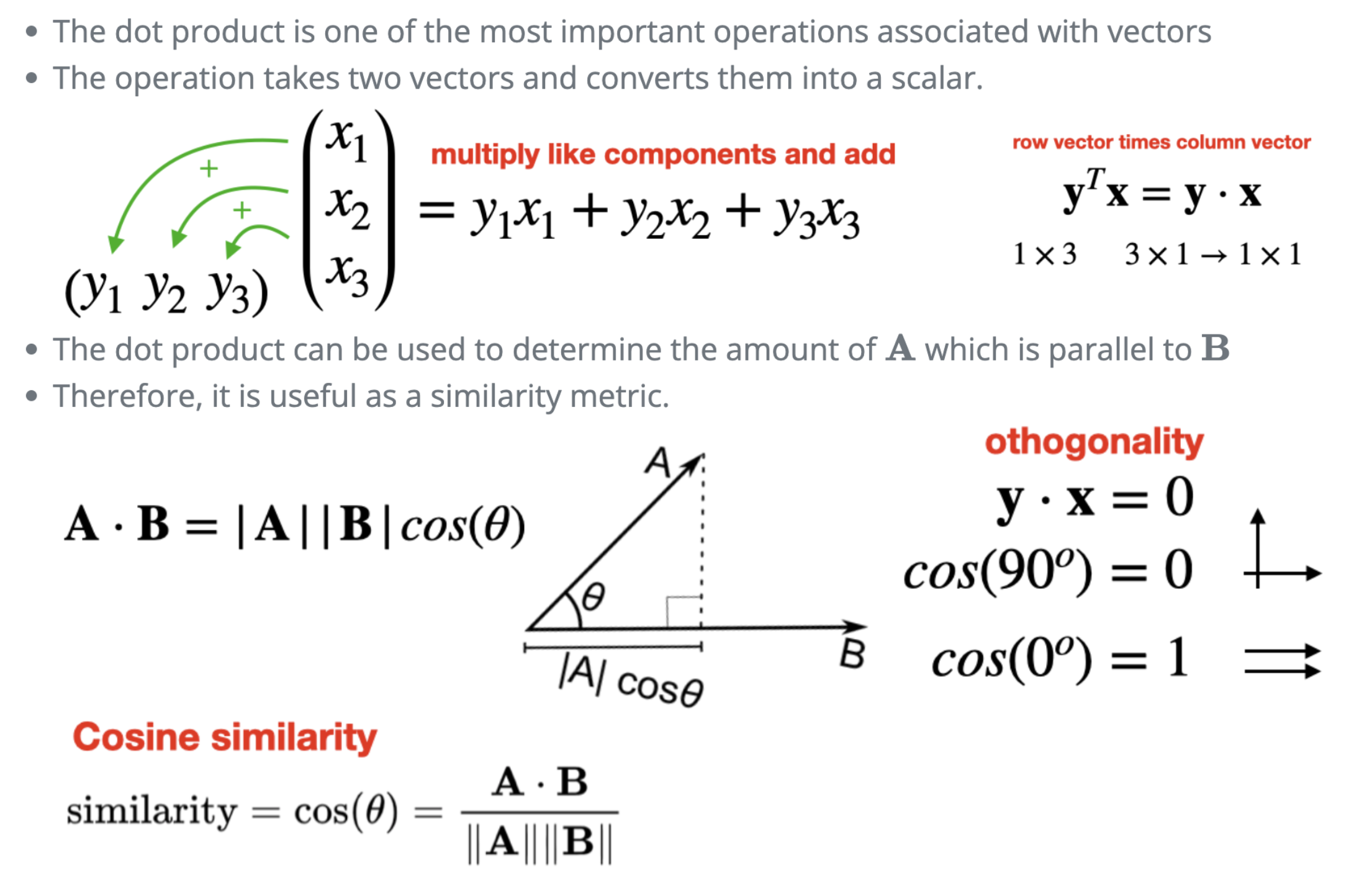
Recall: Inner product
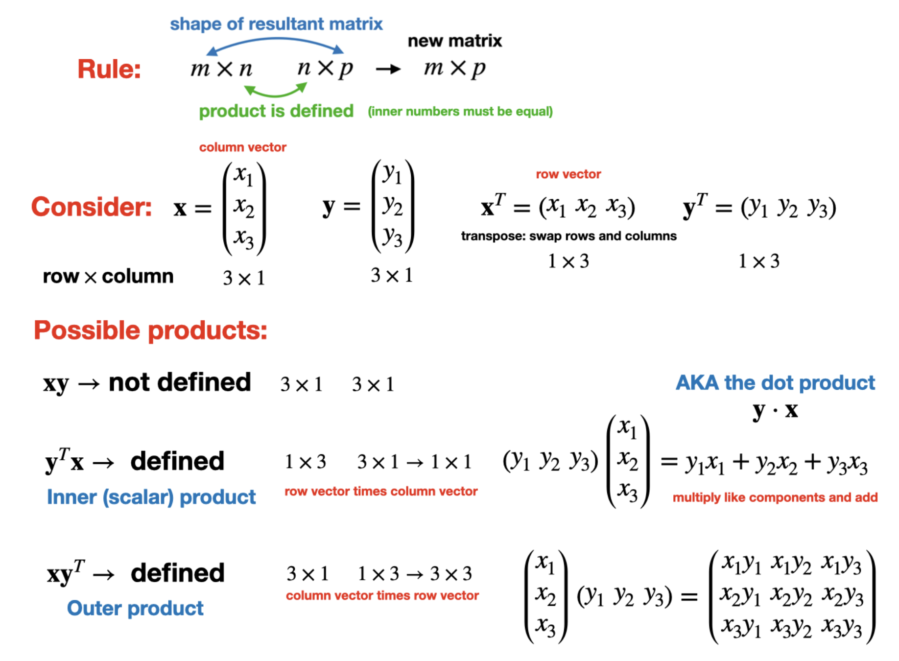
Outer product
Two Matrices you can build from data
Four points, two features. Already centered \((\boldsymbol{\mu}=\mathbf{0})\).
\[ X=\left(\begin{array}{cc} 2 & 1 \\ 1 & 2 \\ -1 & -2 \\ -2 & -1 \end{array}\right) \quad(n=4, d=2) \]
From one data matrix, two very different products:
| Definition | Shape | Indexed by | |
|---|---|---|---|
| Covariance | \(C=X^{\top} X\) | \(d \times d=2 \times 2\) | features |
| Gram | \(G=X X^{\top}\) | \(n \times n=4 \times 4\) | data points |
Same data. One matrix grows with the number of features, the other with the number of observations.
The Covariance Matrix (\(d \times d\))
The Covariance Matrix \((d \times d)\)
\[ C=X^{\top} X=\left(\begin{array}{cc} 10 & 8 \\ 8 & 10 \end{array}\right) \]
Eigendecomposition:The eigenvectors are directions in feature space. \(\mathbf{v}_1\) says “feature 1 and feature 2 move together.” That statement is about the variables, not about Ann or Ben.
PCA come from projecting: \(\mathbf{z}=W^{\top} \mathbf{x}\), giving (2.12, 2.12, -2.12, -2.12) on PC1.
\(W\) is the matrix whose columns are the eigenvectors of \(C\), kept in descending eigenvalue order. It’s \(d \times k\) - features by components.
The Gram Matrix ( \(n \times n\) )
\[ G=X X^{\top}=\left(\begin{array}{cccc} 5 & 4 & -4 & -5 \\ 4 & 5 & -5 & -4 \\ -4 & -5 & 5 & 4 \\ -5 & -4 & 4 & 5 \end{array}\right) \]
Same nonzero spectrum \(-\lambda=18,2\) - but the top eigenvector is
\[ \mathbf{u}_1=\frac{1}{2}(1,1,-1,-1) \]
One entry per data point. This eigenvector is the embedding: it already contains the four coordinates. There is no direction, no \(W\), nothing to apply to anything.
The Gram matrix is named after Jorgen Pedersen Gram, a Danish actuary and mathematician.
Now a Fifth Point Arrives: \(\mathbf{x}_5=(3,2)\)
Covariance route (inductive).
\[ z_1=\mathbf{v}_1^{\top} \mathbf{x}_5=\frac{3+2}{\sqrt{2}}=3.54 \]
Done. \(W\) is \(2 \times 2\) and does not know or care how many points it was estimated from.
Gram route (transductive).
\(G\) is now \(5 \times 5\). Its eigenvectors live in \(\mathbb{R}^5\), not \(\mathbb{R}^4\) - a different vector space. Every existing coordinate is recomputed. There was never a function to evaluate; the coordinates were the parameters.
Fitting more data refines \(W\). Fitting more data replaces \(\mathbf{u}\).
This is why our spectral methods are transductive.
Why Shape Decides Everything
- \(d \times d\) → parameters on the feature axis → a reusable map → inductive
- \(n \times n\) → parameters on the identity axis → one row per training point → transductive
- In t-SNE, Isomap, LLE, and spectral clustering, the \(n \times n\) matrix is built from pairwise distances or affinities, and no \(X\) survives to cross back with. That is what makes them hard-transductive.
The eigendecomposition was never the problem. What the index runs over is the problem.