We can see that this dataset holds exactly one graph,
each node in this dataset is assigned a 34-dimensional feature vector (which uniquely describes the members of the karate club).
Furthermore, the graph holds exactly 4 classes, which represent the community each node belongs to.
Code
from torch_geometric.datasets import KarateClubdataset = KarateClub()print(f'Dataset: {dataset}:')print('======================')print(f'Number of graphs: {len(dataset)}')print(f'Number of features: {dataset.num_features}')print(f'Number of classes: {dataset.num_classes}')
Dataset: KarateClub():
======================
Number of graphs: 1
Number of features: 34
Number of classes: 4
Looking at a data-point
Lets look at the first, and only, graph in the dataset.
Code
data = dataset[0] # Get the first graph object.print(data)print('==============================================================')# Gather some statistics about the graph.print(f'Number of nodes: {data.num_nodes}')print(f'Number of edges: {data.num_edges}')print(f'Average node degree: {data.num_edges / data.num_nodes:.2f}')print(f'Number of training nodes: {data.train_mask.sum()}')print(f'Training node label rate: {int(data.train_mask.sum()) / data.num_nodes:.2f}')print(f'Has isolated nodes: {data.has_isolated_nodes()}')print(f'Has self-loops: {data.has_self_loops()}')print(f'Is undirected: {data.is_undirected()}')
Data(x=[34, 34], edge_index=[2, 156], y=[34], train_mask=[34])
==============================================================
Number of nodes: 34
Number of edges: 156
Average node degree: 4.59
Number of training nodes: 4
Training node label rate: 0.12
Has isolated nodes: False
Has self-loops: False
Is undirected: True
Training mask
The additional attribute called train_mask, which describes for which nodes we already know their community assignments.
In total, we are only aware of the ground-truth labels of 4 nodes (one for each community), and the task is to infer the community assignment for the remaining nodes.
Code
# optional add more training points# random sample 10 training pointsindices=torch.randperm(data.num_nodes)[:int(0.5*data.num_nodes)]data.train_mask[:] =Falsedata.train_mask[indices] =True# printprint(data.train_mask)print("len(data.train_mask):",sum(data.train_mask[data.train_mask==True])/len(data.train_mask))print(f'Number of nodes in Graph[0]: {dataset[0].num_nodes}')print(f'Number of edges in Graph[0]: {dataset[0].num_edges}')
tensor([False, False, False, False, False, False,  True,  True, False,  True,
         True,  True, False, False,  True,  True,  True, False,  True, False,
         True, False,  True,  True, False, False, False, False,  True,  True,
         True,  True,  True, False])
len(data.train_mask): tensor(0.5000)
Number of nodes in Graph[0]: 34
Number of edges in Graph[0]: 156
Data objects
Let us now inspect the edge_index property in more detail:
Code
# from IPython.display import Javascript # Restrict height of output cell.# display(Javascript('''google.colab.output.setIframeHeight(0, true, {maxHeight: 300})'''))edge_index = data.edge_indexprint(edge_index.shape)# print(edge_index.t())
torch.Size([2, 156])
Explore target labels
Notice how there are 34 targets, one for each node.
Often there are only two classes (administrator, instructor), however in this case there are 4.
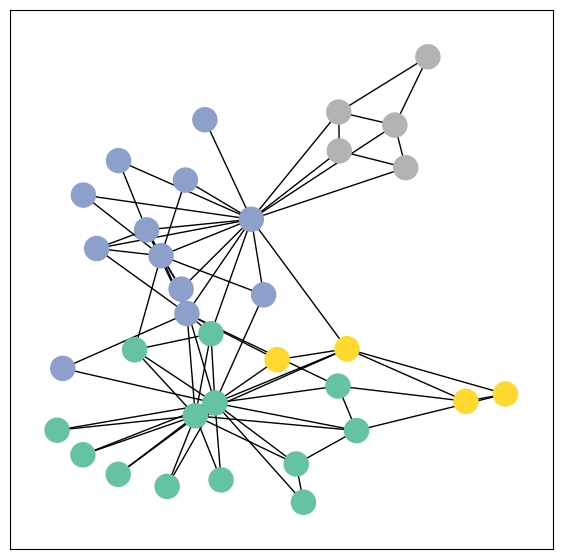
Class 0: Members loyal to Mr. Hi (the club administrator).
Class 1: Members loyal to John A. (the instructor).
Class 2: Members who are more closely associated with Mr. Hi’s group but not as central.
Class 3: Members who are more closely associated with John A.’s group but not as central.
from torch_geometric.utils import to_networkxG = to_networkx(data, to_undirected=True)# color code based on group labels visualize_graph(G, color=data.y)
Coding the GNN model
The GCN model stacks three GCNConv layers (with tanh activations) to aggregate 3-hop neighborhood information, reducing features from 34 → 4 → 4 → 2.
A final Linear layer classifies nodes into 4 classes.
The model returns both class scores and final node embeddings.
Initializing and printing GCN() shows its architecture.
Code
# Define a simple 3-layer GCN model for node classification.import torchfrom torch.nn import Linearfrom torch_geometric.nn import GCNConvclass GCN(torch.nn.Module):def__init__(self):super().__init__() torch.manual_seed(12345) # Set random seed for reproducibilityself.conv1 = GCNConv(dataset.num_features, 4) # First GCN layer: input features -> 4self.conv2 = GCNConv(4, 4) # Second GCN layer: 4 -> 4self.conv3 = GCNConv(4, 2) # Third GCN layer: 4 -> 2# REMEMBER THAT IN PYTORCH CCE LOSS APPLIES SOFTMAX AUTOMATICALLYself.classifier = Linear(2, dataset.num_classes) # Final linear classifier: 2 -> num_classesdef forward(self, x, edge_index): h =self.conv1(x, edge_index) h = h.tanh() # Nonlinearity after first layer h =self.conv2(h, edge_index) h = h.tanh() # Nonlinearity after second layer h =self.conv3(h, edge_index) h = h.tanh() # Nonlinearity after third layer (final embedding)# Apply a final (linear) classifier to the embeddings. out =self.classifier(h)return out, h # Return class scores and embeddingsmodel = GCN()print(model)
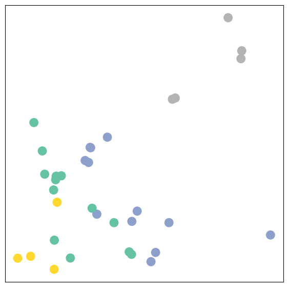
Let’s take a look at the INITIAL (untrained) node embeddings produced by our GNN.
Here, we pass in the initial node features x and the graph connectivity information edge_index to the model, and visualize its 2-dimensional embedding.
Code
model = GCN()# h is the final hidden state representation before sending to classifier o, h = model(data.x, data.edge_index)print(f'Embedding shape: {list(h.shape)}')print(f'Classifier output shape: {list(o.shape)}')visualize_embedding(h, color=data.y)
Inductive bias is the set of assumptions a learning algorithm uses to generalize to unseen data.
Even before training, our model’s random weights produce node embeddings that already reflect the graph’s community structure.
Nodes from the same community cluster together in the embedding space, despite no training.
This shows GNNs have a strong inductive bias, making nearby nodes in the graph have similar embeddings.
Inductive vs Transductive
Transductive GNNs
Train and test on the same graph
Goal: predict labels for unlabeled nodes within that graph
The full graph structure is known during training
Example: Cora citation dataset with masked node labels
Inductive GNNs
Train on one graph (or set of graphs) and generalize to unseen graphs or nodes
Goal: make predictions on new nodes or graphs not seen during training
Model must learn transferable patterns
Example: predicting protein functions on new protein interaction networks
Training
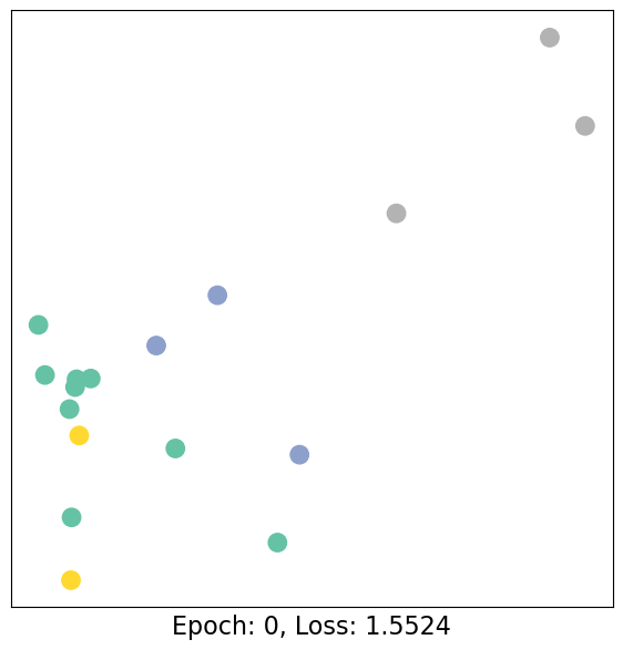
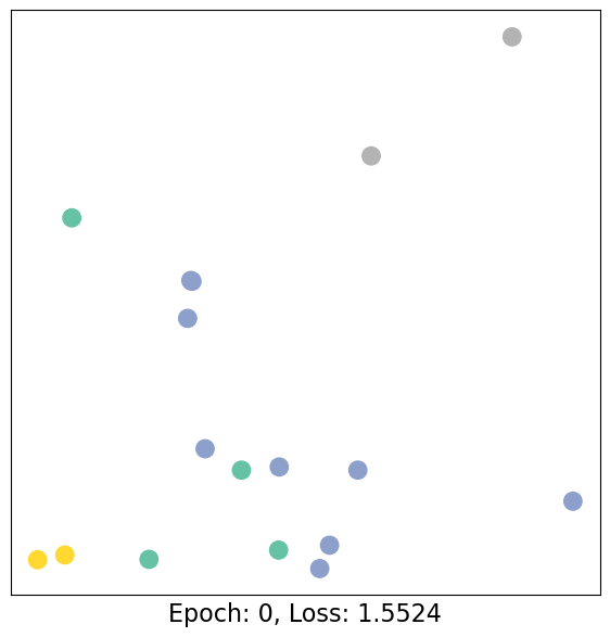
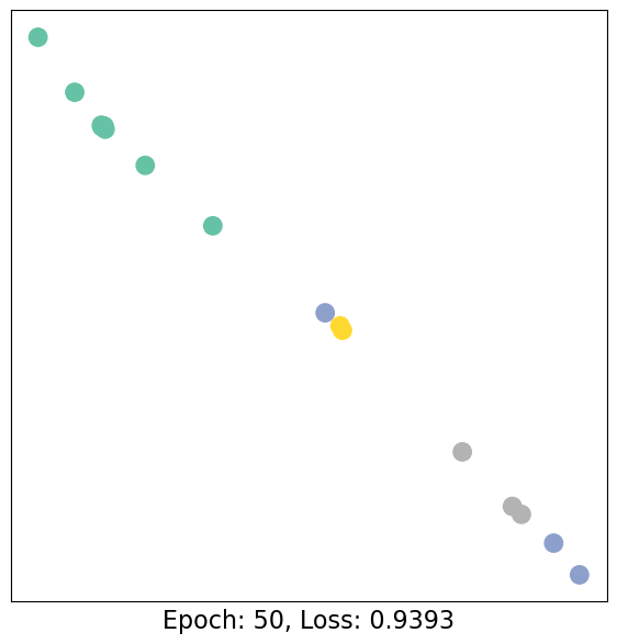
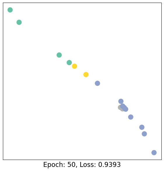
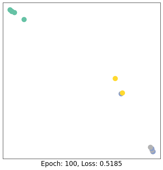
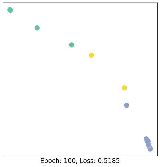
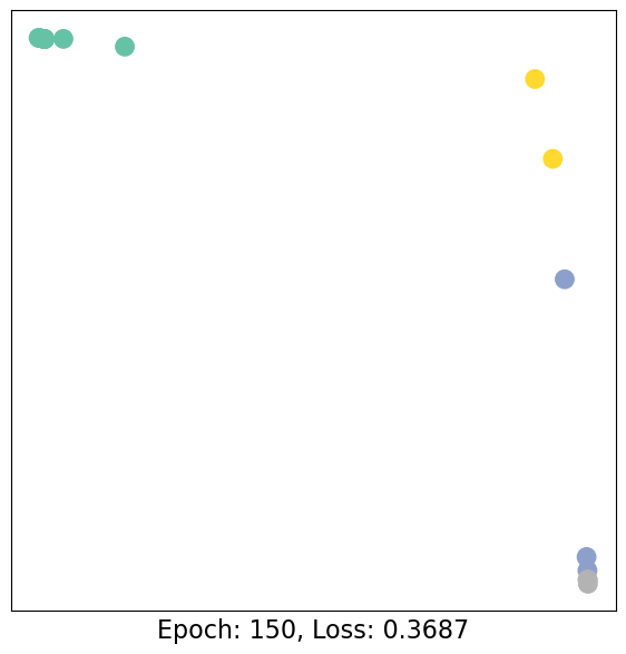
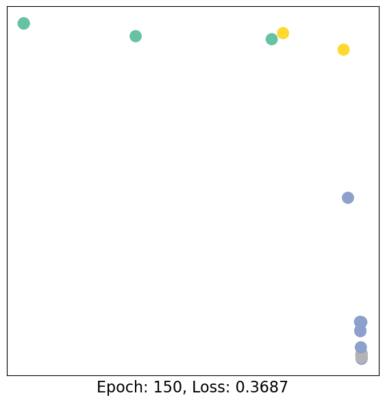
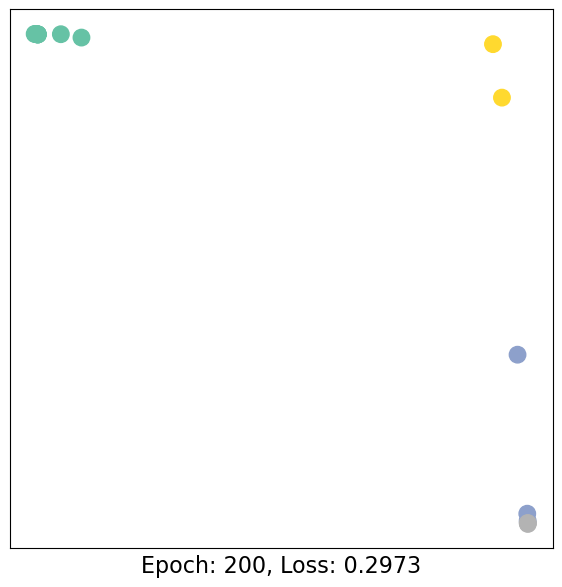
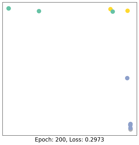
Training on the Karate Club Network involves updating the model parameters using known community assignments for 4 nodes (one from each community).
The model is fully differentiable and parameterized, allowing us to add labels and observe how node embeddings change during training.
A semi-supervised (transductive) learning approach is used: training is performed on one labeled node per class, while the entire graph structure is available as input.
Training details
Training follows standard PyTorch workflow:
Define network architecture, loss function (CrossEntropyLoss), and optimizer (Adam)
Perform multiple optimization rounds with forward and backward passes
Semi-supervised learning is implemented by computing loss only on training nodes:
loss = criterion(out[data.train_mask], data.y[data.train_mask])
Node embeddings are computed for all nodes, but only training nodes contribute to the loss
Training allows us to observe how node embeddings evolve over time
This works since softmax is monotonic, which means that the order of the logits is preserved after applying softmax.
If you want the class probabilities:
probs = torch.softmax(logits, dim=1)
Note on pytorch CrossEntropyLoss
PyTorch’s torch.nn.CrossEntropyLoss avoids needing a softmax + OHE by combining everything into one mathematically equivalent operation. Here’s how it works:
logits: shape [N, C] — raw, unnormalized scores from the model.
target: shape [N] — integer class labels (e.g., [0, 2, 1, 3]), not one-hot encoded.
PyTorch’s CrossEntropyLoss is mathematically equivalent to doing softmax followed by comparing with one-hot targets, but it does it in a numerically stable and efficient way by combining log_softmax + NLL in one step.
Code: Training our model
Code
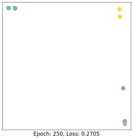
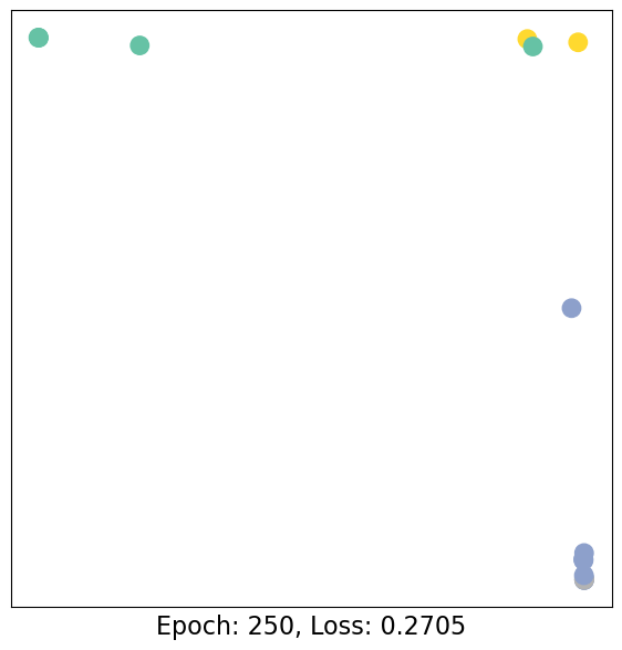
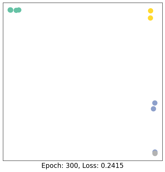
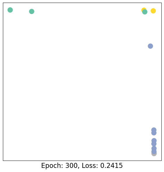
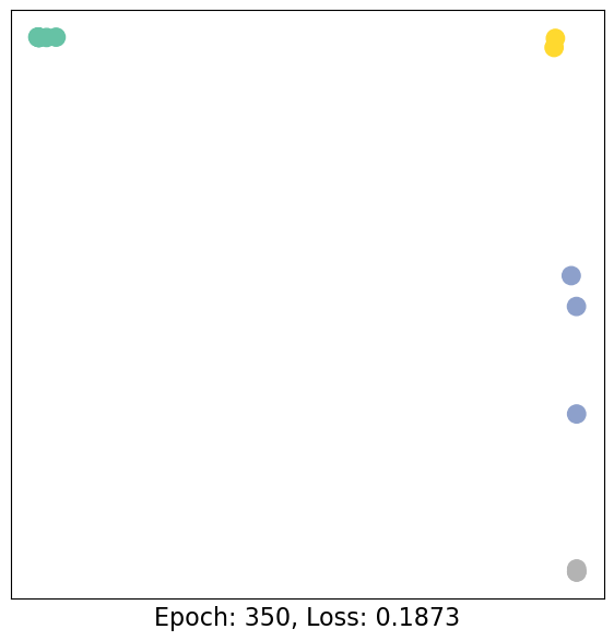
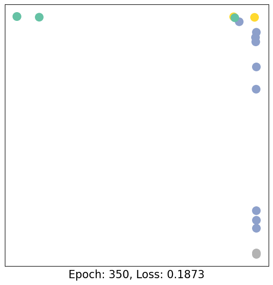
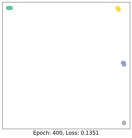
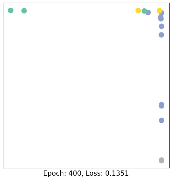
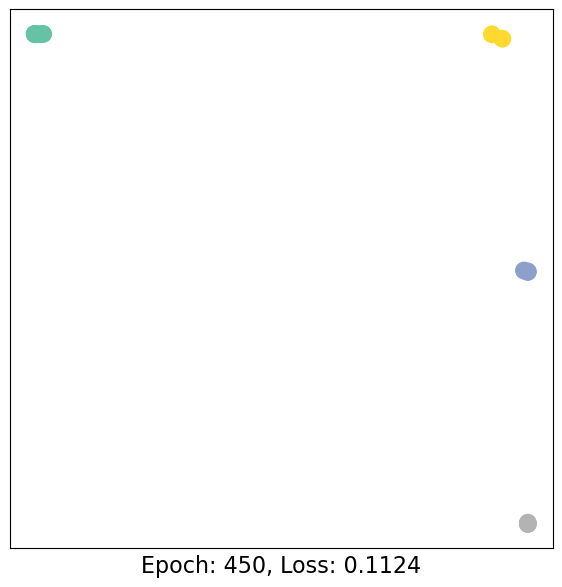
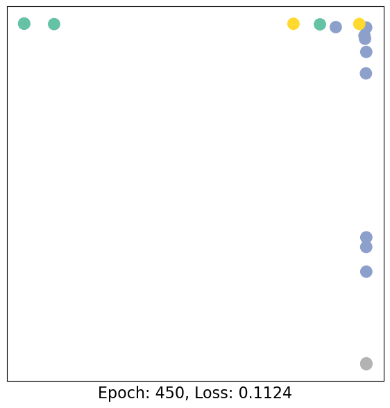
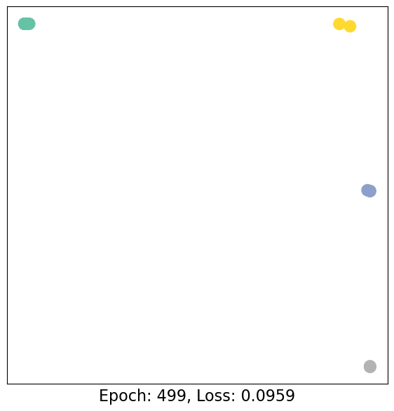
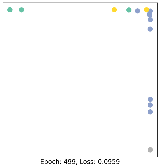
import time# initialize model = GCN()criterion = torch.nn.CrossEntropyLoss() # Define loss criterion.optimizer = torch.optim.Adam(model.parameters(), lr=0.01) # Define optimizer.# training loopepochs=[]acc_train=[] acc_val=[] losses=[]losses_val=[]num_epochs=500for epoch inrange(num_epochs): optimizer.zero_grad() # Clear gradients. out, h = model(data.x, data.edge_index) # Perform a single forward pass.# training accuracy yt_pred = torch.argmax(out[data.train_mask], dim=1) yt_true = data.y[data.train_mask] acc_train.append(torch.sum(yt_pred == yt_true) /len(yt_pred))# validation accuracy yv_pred = torch.argmax(out[data.train_mask==False], dim=1) yv_true = data.y[data.train_mask==False] acc_val.append(torch.sum(yv_pred == yv_true) /len(yv_pred)) epochs.append(epoch) loss = criterion(out[data.train_mask], data.y[data.train_mask]) # Compute the loss solely based on the training nodes. losses.append(loss.item()) loss.backward() # Derive gradients. optimizer.step() # Update parameters based on gradients. loss_val = criterion(out[data.train_mask==False], data.y[data.train_mask==False]) # Compute the loss solely based on the training nodes. losses_val.append(loss_val.item())if epoch %50==0or epoch == num_epochs-1:print(f"Epoch {epoch} of {num_epochs}")print("Shapes")print(data.x.shape, h.shape, out.shape,data.y.shape)print(out[data.train_mask].shape, data.y[data.train_mask].shape)print(out[data.train_mask==False].shape, data.y[data.train_mask==False].shape)print(yt_pred, yt_true)print(yv_pred, yv_true)print("------------TRAINING------------") visualize_embedding(h[data.train_mask], color=data.y[data.train_mask], epoch=epoch, loss=loss)print("------------VALIDATION------------") visualize_embedding(h[data.train_mask==False], color=data.y[data.train_mask==False] , epoch=epoch, loss=loss) time.sleep(0.3)
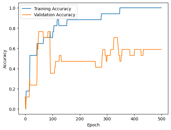
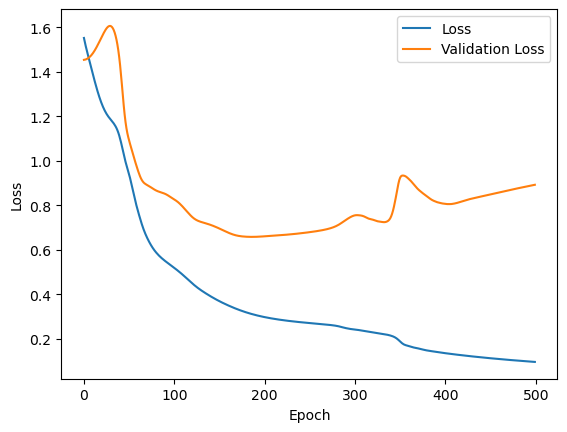
# plot the accuracyplt.plot(epochs, acc_train, label='Training Accuracy')plt.plot(epochs, acc_val, label='Validation Accuracy')plt.xlabel('Epoch')plt.ylabel('Accuracy')plt.legend()plt.show()# plot the lossplt.plot(epochs, losses, label='Loss')plt.plot(epochs, losses_val, label='Validation Loss')plt.xlabel('Epoch')plt.ylabel('Loss')plt.legend()plt.show()
Results
As one can see, our 3-layer GCN model manages to linearly separating the communities and classifying most of the nodes correctly.
Furthermore, we did this all with a few lines of code, thanks to the PyTorch Geometric library which helped us out with data handling and GNN implementations.
Conclusion
This concludes the first introduction into the world of GNNs and PyTorch Geometric. In the follow-up sessions, you will learn how to achieve state-of-the-art classification results on a number of real-world graph datasets.