Code
2.6.0.dev20240722The following is a recording on this topic, I hope you find it useful!
Feel free to watch at 1.5x or 2x speed.
Note: If you find something missing or incorrect in the recording, then please let me know!
Recently, deep learning on graphs has emerged to one of the hottest research fields in the deep learning community.
Graph Neural Networks (GNNs) aim to generalize classical deep learning concepts to irregular structured data (in contrast to images or texts) and to enable neural networks to reason about objects and their relations.
This is done by following a neural message passing scheme, where node features \(\mathbf{x}_v^{(\ell)}\) of all nodes \(v \in \mathcal{V}\) in a graph \(\mathcal{G} = (\mathcal{V}, \mathcal{E})\) are iteratively updated by aggregating localized information from their neighbors \(\mathcal{N}(v)\):
\[ \mathbf{x}_v^{(\ell + 1)} = f^{(\ell + 1)}_{\theta} \left( \mathbf{x}_v^{(\ell)}, \left\{ \mathbf{x}_w^{(\ell)} : w \in \mathcal{N}(v) \right\} \right) \]
At its core, PyG provides the following main features:
Data Handling of Graphs in PyG
torch_geometric.dataData] object, which holds all the information to describe its graph representation.instance of torch_geometric.data.data.x : Node feature matrix with shape [num_nodes, num_node_features]data.edge_index : Graph connectivity in COO format with shape [2, num_edges] and type torch.longdata.edge_attr : Edge feature matrix with shape [num_edges, num_edge_features]data.y : Target to train against (may have arbitrary shape), e.g., node-level targets of shape [num_nodes, *] or graph-level targets of shape [1, *]data.pos : Node position matrix with shape [num_nodes, num_dimensions]None of these attributes are strictly required.
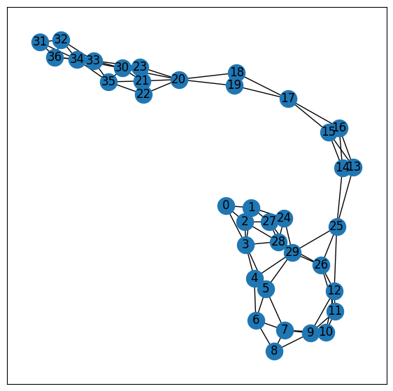
torch_geometric.data: Closer lookprint(data) provides a short summary about its attributes and their shapes:Data(edge_index=[2, 156], x=[34, 34], y=[34], train_mask=[34])data object holds 4 attributes:
edge_index property holds the information about the graph connectivity, i.e., a tuple of source and destination node indices for each edge.x (each of the 34 nodes is assigned a 34-dim feature vector), and toy (each node is assigned to exactly one class).train_mask, which describes for which nodes we already know their community assignments.The data object also provides some utility functions to infer some basic properties of the underlying graph.
For example, we can easily infer whether there exists isolated nodes in the graph (i.e. there exists no edge to any node), whether the graph contains self-loops (i.e., \((v, v) \in \mathcal{E}\)), or whether the graph is undirected (i.e., for each edge \((v, w) \in \mathcal{E}\) there also exists the edge \((w, v) \in \mathcal{E}\)).
edge_index holds tuples of source and destination node indices.networkx for advanced visualization and graph manipulation.For more details, visit the PyTorch Geometric documentation.
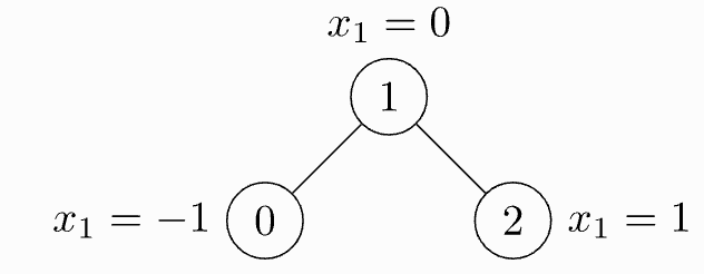
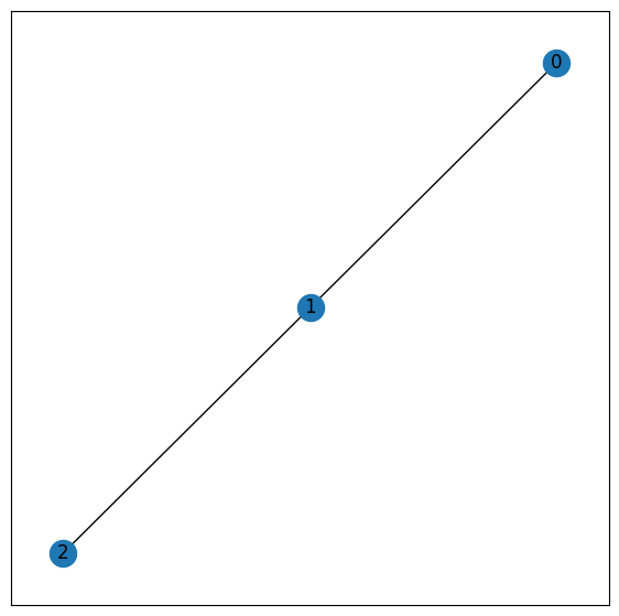
data.edge_index : Graph connectivity in COO format with shape [2, num_edges] and type torch.longedge_index = torch.tensor([[0, 1, 1, 2], [1, 0, 2, 1]], dtype=torch.long)import torch
from torch_geometric.data import Data
# basically an edge list representation
# [[source],[target]]
# source [0, 1, 1, 2]--> target [1, 0, 2, 1]
edge_index = torch.tensor([[0, 1, 1, 2], [1, 0, 2, 1]], dtype=torch.long)
# Feature vector
x = torch.tensor([[-1], [0], [1]], dtype=torch.float)
# Type cast into
data = Data(x=x, edge_index=edge_index)
print(type(data))
print("shapes =",data)
print(data.x)
print(data.edge_index)
print(data.edge_index.T)<class 'torch_geometric.data.data.Data'>
shapes = Data(x=[3, 1], edge_index=[2, 4])
tensor([[-1.],
[ 0.],
[ 1.]])
tensor([[0, 1, 1, 2],
[1, 0, 2, 1]])
tensor([[0, 1],
[1, 0],
[1, 2],
[2, 1]])you should transpose and call contiguous before passing them to the data constructor:
.contiguous() in PyTorch ensures that a tensor is stored in contiguous memory, allowing for more efficient operations and easier reshaping.edge_index labeling & Validate()The Data object provides a number of useful utility functions, e.g.:
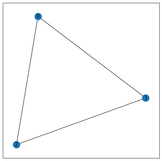
shapes = Data(x=[3, 1], edge_index=[2, 6])
<class 'torch_geometric.data.data.Data'>
tensor([[-1.],
        [ 0.],
        [ 1.]])
tensor([[0, 1, 0, 2, 1, 2],
[1, 0, 2, 0, 2, 1]])https://pytorch-geometric.readthedocs.io/en/latest/generated/torch_geometric.data.Data.html#torch_geometric.data.Data
['__abstractmethods__', '__annotations__', '__call__', '__cat_dim__', '__class__', '__contains__', '__copy__', '__deepcopy__', '__delattr__', '__delitem__', '__dict__', '__dir__', '__doc__', '__eq__', '__format__', '__ge__', '__getattr__', '__getattribute__', '__getitem__', '__getstate__', '__gt__', '__hash__', '__inc__', '__init__', '__init_subclass__', '__iter__', '__le__', '__len__', '__lt__', '__module__', '__ne__', '__new__', '__reduce__', '__reduce_ex__', '__repr__', '__setattr__', '__setitem__', '__setstate__', '__sizeof__', '__slots__', '__str__', '__subclasshook__', '__weakref__', '_abc_impl', '_edge_attr_cls', '_edge_to_layout', '_edges_to_layout', '_get_edge_index', '_get_tensor', '_get_tensor_size', '_multi_get_tensor', '_put_edge_index', '_put_tensor', '_remove_edge_index', '_remove_tensor', '_store', '_tensor_attr_cls', '_to_type', 'apply', 'apply_', 'batch', 'clone', 'coalesce', 'concat', 'contains_isolated_nodes', 'contains_self_loops', 'contiguous', 'coo', 'cpu', 'csc', 'csr', 'cuda', 'debug', 'detach', 'detach_', 'edge_attr', 'edge_attrs', 'edge_index', 'edge_stores', 'edge_subgraph', 'edge_weight', 'face', 'from_dict', 'generate_ids', 'get_all_edge_attrs', 'get_all_tensor_attrs', 'get_edge_index', 'get_tensor', 'get_tensor_size', 'has_isolated_nodes', 'has_self_loops', 'is_coalesced', 'is_cuda', 'is_directed', 'is_edge_attr', 'is_node_attr', 'is_sorted', 'is_sorted_by_time', 'is_undirected', 'keys', 'multi_get_tensor', 'node_attrs', 'node_offsets', 'node_stores', 'num_edge_features', 'num_edge_types', 'num_edges', 'num_faces', 'num_features', 'num_node_features', 'num_node_types', 'num_nodes', 'pin_memory', 'pos', 'put_edge_index', 'put_tensor', 'record_stream', 'remove_edge_index', 'remove_tensor', 'requires_grad_', 'share_memory_', 'size', 'snapshot', 'sort', 'sort_by_time', 'stores', 'stores_as', 'subgraph', 'time', 'to', 'to_dict', 'to_heterogeneous', 'to_namedtuple', 'up_to', 'update', 'update_tensor', 'validate', 'view', 'x', 'y']['__call__', '__cat_dim__', '__class__', '__contains__', '__copy__', '__deepcopy__', '__delattr__', '__delitem__', '__dir__', '__eq__', '__format__', '__ge__', '__getattr__', '__getattribute__', '__getitem__', '__getstate__', '__gt__', '__inc__', '__init__', '__init_subclass__', '__iter__', '__le__', '__len__', '__lt__', '__ne__', '__new__', '__reduce__', '__reduce_ex__', '__repr__', '__setattr__', '__setitem__', '__setstate__', '__sizeof__', '__str__', '__subclasshook__', '__weakref__', '_edge_attr_cls', '_edge_to_layout', '_edges_to_layout', '_get_edge_index', '_get_tensor', '_get_tensor_size', '_multi_get_tensor', '_put_edge_index', '_put_tensor', '_remove_edge_index', '_remove_tensor', '_tensor_attr_cls', '_to_type', 'apply', 'apply_', 'clone', 'coalesce', 'concat', 'contains_isolated_nodes', 'contains_self_loops', 'contiguous', 'coo', 'cpu', 'csc', 'csr', 'cuda', 'debug', 'detach', 'detach_', 'edge_attrs', 'edge_subgraph', 'from_dict', 'generate_ids', 'get_all_edge_attrs', 'get_all_tensor_attrs', 'get_edge_index', 'get_tensor', 'get_tensor_size', 'has_isolated_nodes', 'has_self_loops', 'is_coalesced', 'is_directed', 'is_edge_attr', 'is_node_attr', 'is_sorted', 'is_sorted_by_time', 'is_undirected', 'keys', 'multi_get_tensor', 'node_attrs', 'pin_memory', 'put_edge_index', 'put_tensor', 'record_stream', 'remove_edge_index', 'remove_tensor', 'requires_grad_', 'share_memory_', 'size', 'snapshot', 'sort', 'sort_by_time', 'stores_as', 'subgraph', 'to', 'to_dict', 'to_heterogeneous', 'to_namedtuple', 'up_to', 'update', 'update_tensor', 'validate', 'view']For more details, visit the PyTorch Geometric documentation.
For more details, visit the PyTorch Geometric documentation.
For more details, visit the PyTorch Geometric documentation.
from torch_geometric.datasets import TUDataset

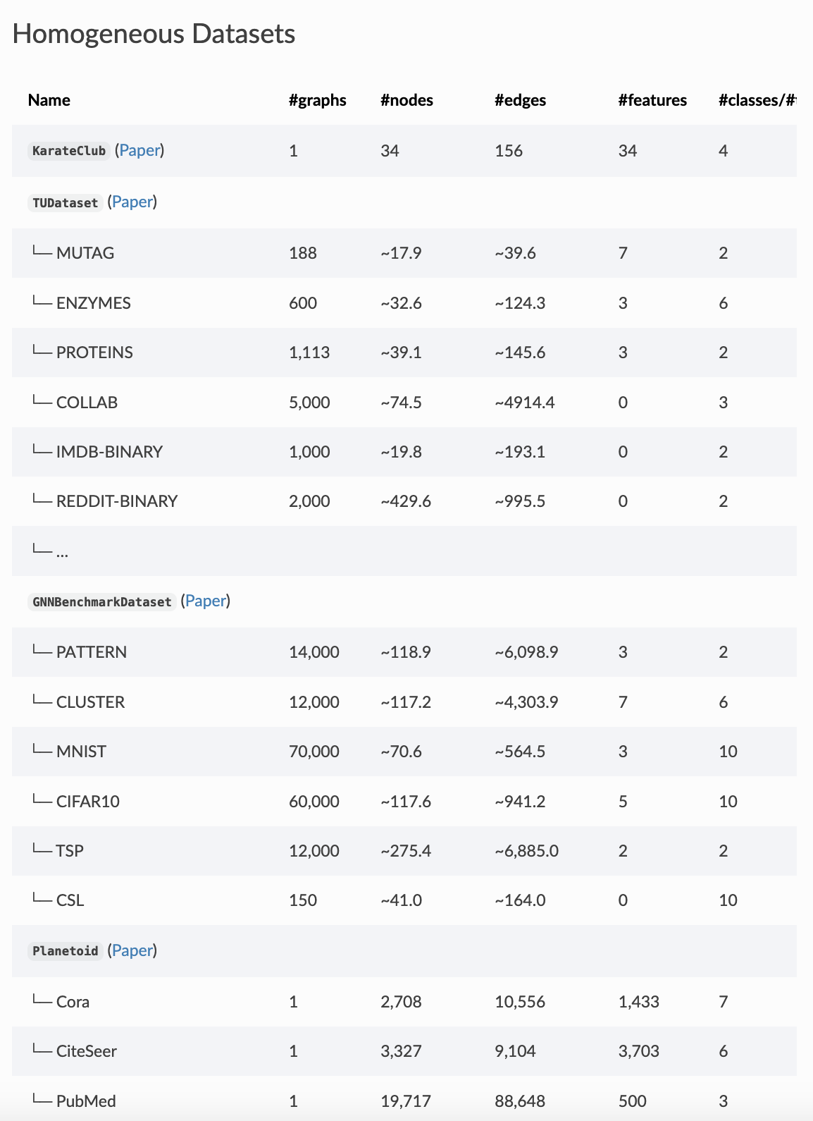
dataset = TUDataset(root='/tmp/ENZYMES', name='ENZYMES')
print("type : ",type(dataset))
print("Number of graphs : ",len(dataset))
print("Number of nodal features : ",dataset.num_node_features)
print("Number of edge features : ",dataset.num_edge_features)
# print("y : ",dataset.y)
print("Number of labels (y) : ",len(dataset.y))
print("Number of classes : ",dataset.num_classes)
type : <class 'torch_geometric.datasets.tu_dataset.TUDataset'>
Number of graphs : 600
Number of nodal features : 3
Number of edge features : 0
Number of labels (y) : 600
Number of classes : 6print("------------------")
print("type : ",type(dataset[0]))
print("shapes: ",dataset[0])
print("Number of nodes : ",dataset[0].num_nodes)
print("Number of edges : ",dataset[0].num_edges)
print("x matrix : \n",dataset[0].x)
print("y label : ",dataset.y[0])
print("Edge List : \n",dataset[0].edge_index)------------------
type : <class 'torch_geometric.data.data.Data'>
shapes: Data(edge_index=[2, 168], x=[37, 3], y=[1])
Number of nodes : 37
Number of edges : 168
x matrix :
tensor([[1., 0., 0.],
[1., 0., 0.],
[1., 0., 0.],
[1., 0., 0.],
[1., 0., 0.],
[1., 0., 0.],
[1., 0., 0.],
[1., 0., 0.],
[1., 0., 0.],
[1., 0., 0.],
[1., 0., 0.],
[1., 0., 0.],
[1., 0., 0.],
[1., 0., 0.],
[1., 0., 0.],
[1., 0., 0.],
[1., 0., 0.],
[1., 0., 0.],
[1., 0., 0.],
[1., 0., 0.],
[1., 0., 0.],
[1., 0., 0.],
[1., 0., 0.],
[1., 0., 0.],
[0., 1., 0.],
[0., 1., 0.],
[0., 1., 0.],
[0., 1., 0.],
[0., 1., 0.],
[0., 1., 0.],
[0., 1., 0.],
[0., 1., 0.],
[0., 1., 0.],
[0., 1., 0.],
[0., 1., 0.],
[0., 1., 0.],
[0., 1., 0.]])
y label : tensor(5)
Edge List :
tensor([[ 0, 0, 0, 1, 1, 1, 1, 1, 2, 2, 2, 2, 2, 3, 3, 3, 3, 3,
3, 4, 4, 4, 4, 5, 5, 5, 5, 5, 6, 6, 6, 6, 7, 7, 7, 7,
7, 8, 8, 8, 9, 9, 9, 9, 9, 10, 10, 10, 10, 11, 11, 11, 11, 12,
12, 12, 12, 12, 13, 13, 13, 13, 14, 14, 14, 14, 15, 15, 15, 15, 16, 16,
16, 16, 17, 17, 17, 17, 18, 18, 18, 19, 19, 19, 20, 20, 20, 20, 20, 20,
21, 21, 21, 21, 21, 22, 22, 22, 22, 23, 23, 23, 23, 24, 24, 24, 24, 25,
25, 25, 25, 25, 26, 26, 26, 26, 26, 27, 27, 27, 27, 27, 28, 28, 28, 28,
28, 28, 29, 29, 29, 29, 29, 29, 29, 30, 30, 30, 30, 30, 31, 31, 31, 32,
32, 32, 32, 33, 33, 33, 33, 33, 33, 34, 34, 34, 34, 34, 34, 35, 35, 35,
35, 35, 36, 36, 36, 36],
[ 1, 2, 3, 0, 2, 3, 24, 27, 0, 1, 3, 27, 28, 0, 1, 2, 4, 5,
28, 3, 5, 6, 29, 3, 4, 6, 7, 29, 4, 5, 7, 8, 5, 6, 8, 9,
10, 6, 7, 9, 7, 8, 10, 11, 12, 7, 9, 11, 12, 9, 10, 12, 26, 9,
10, 11, 25, 26, 14, 15, 16, 25, 13, 15, 16, 25, 13, 14, 16, 17, 13, 14,
15, 17, 15, 16, 18, 19, 17, 19, 20, 17, 18, 20, 18, 19, 21, 22, 23, 30,
20, 22, 23, 30, 35, 20, 21, 23, 35, 20, 21, 22, 33, 1, 27, 28, 29, 12,
13, 14, 26, 29, 11, 12, 25, 28, 29, 1, 2, 24, 28, 29, 2, 3, 24, 26,
27, 29, 4, 5, 24, 25, 26, 27, 28, 20, 21, 33, 34, 35, 32, 34, 36, 31,
33, 34, 36, 23, 30, 32, 34, 35, 36, 30, 31, 32, 33, 35, 36, 21, 22, 30,
33, 34, 31, 32, 33, 34]])Lets combine some of that code into a utility function
def dataset_summary(dataset):
print("---------- Data Set Properties ----------")
print("type : ",type(dataset))
print("Number of graphs : ",len(dataset))
print("Number of nodal features : ",dataset.num_node_features)
print("Number of edge features : ",dataset.num_edge_features)
# print("y : ",dataset.y)
print("Number of labels (y) : ",len(dataset.y))
print("Number of classes : ",dataset.num_classes)
print("---------- Misc Graph Properties ----------")
#randomize
dataset = dataset.shuffle()
max_index=min(len(dataset),3)
for i in range(0,max_index):
print("------------------")
print("type : ",type(dataset[i]))
print("shapes: ",dataset[i])
print("Number of nodes : ",dataset[i].num_nodes)
print("Number of edges : ",dataset[i].num_edges)
print("x matrix size: \n",dataset[i].x.shape)
print("y label : ",dataset.y[i])
print("Edge List size: \n",dataset[i].edge_index.shape)
dataset_summary(dataset)---------- Data Set Properties ----------
type :  <class 'torch_geometric.datasets.tu_dataset.TUDataset'>
Number of graphs :  600
Number of nodal features :  3
Number of edge features :  0
Number of labels (y) :  600
Number of classes :  6
---------- Misc Graph Properties ----------
------------------
type : <class 'torch_geometric.data.data.Data'>
shapes: Data(edge_index=[2, 122], x=[32, 3], y=[1])
Number of nodes : 32
Number of edges : 122
x matrix size:
torch.Size([32, 3])
y label : tensor(2)
Edge List size:
torch.Size([2, 122])
------------------
type : <class 'torch_geometric.data.data.Data'>
shapes: Data(edge_index=[2, 116], x=[27, 3], y=[1])
Number of nodes : 27
Number of edges : 116
x matrix size:
torch.Size([27, 3])
y label : tensor(1)
Edge List size:
torch.Size([2, 116])
------------------
type : <class 'torch_geometric.data.data.Data'>
shapes: Data(edge_index=[2, 104], x=[30, 3], y=[1])
Number of nodes : 30
Number of edges : 104
x matrix size:
torch.Size([30, 3])
y label : tensor(1)
Edge List size:
torch.Size([2, 104])# Transfer data object to GPU.
device = torch.device('cuda')
data = data.to(device)If you are unsure whether the dataset is already shuffled before you split, you can randomly permutate it by running:
We can use slices, long or bool tensors to split the dataset. E.g., to create a 90/10 train/test split, type:
This is equivalent of doing:
---------- Data Set Properties ----------
type :  <class 'torch_geometric.datasets.planetoid.Planetoid'>
Number of graphs :  1
Number of nodal features :  1433
Number of edge features :  0
Number of labels (y) :  2708
Number of classes :  7
---------- Misc Graph Properties ----------
------------------
type :  <class 'torch_geometric.data.data.Data'>
shapes:  Data(x=[2708, 1433], edge_index=[2, 10556], y=[2708], train_mask=[2708], val_mask=[2708], test_mask=[2708])
Number of nodes :  2708
Number of edges :  10556
x matrix size:
 torch.Size([2708, 1433])
y label :  tensor(3)
Edge List size:
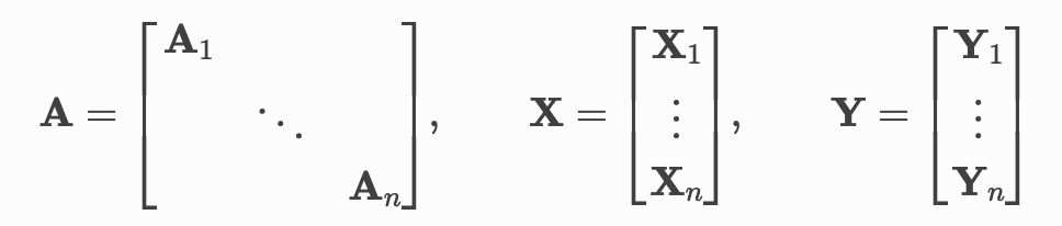
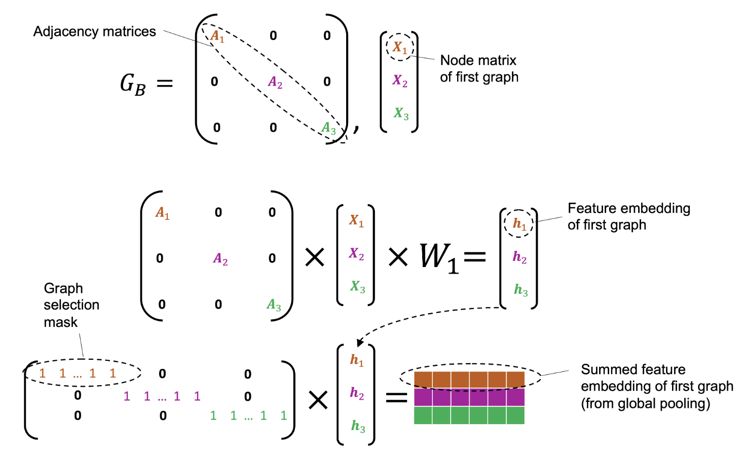
torch.Size([2, 10556])torch_geometric.loader.DataLoadertorch_geometric.data.Batch inherits from torch_geometric.data.Data and contains an additional attribute called batch.
from torch_geometric.datasets import TUDataset
from torch_geometric.loader import DataLoader

dataset = TUDataset(root='/tmp/ENZYMES', name='ENZYMES', use_node_attr=True)
loader = DataLoader(dataset, batch_size=32, shuffle=True)

for batch in loader:
    # print(len(batch))
    print(batch)
    print(batch.num_graphs)

# for batch in loader:
#     print(batch.batch[0])
DataBatch(edge_index=[2, 4114], x=[1047, 21], y=[32], batch=[1047], ptr=[33])
32
DataBatch(edge_index=[2, 4184], x=[1062, 21], y=[32], batch=[1062], ptr=[33])
32
DataBatch(edge_index=[2, 3770], x=[962, 21], y=[32], batch=[962], ptr=[33])
32
DataBatch(edge_index=[2, 4160], x=[1145, 21], y=[32], batch=[1145], ptr=[33])
32
DataBatch(edge_index=[2, 4158], x=[1080, 21], y=[32], batch=[1080], ptr=[33])
32
DataBatch(edge_index=[2, 3884], x=[984, 21], y=[32], batch=[984], ptr=[33])
32
DataBatch(edge_index=[2, 3738], x=[1071, 21], y=[32], batch=[1071], ptr=[33])
32
DataBatch(edge_index=[2, 3886], x=[985, 21], y=[32], batch=[985], ptr=[33])
32
DataBatch(edge_index=[2, 3846], x=[1098, 21], y=[32], batch=[1098], ptr=[33])
32
DataBatch(edge_index=[2, 4306], x=[1222, 21], y=[32], batch=[1222], ptr=[33])
32
DataBatch(edge_index=[2, 3860], x=[988, 21], y=[32], batch=[988], ptr=[33])
32
DataBatch(edge_index=[2, 4190], x=[1072, 21], y=[32], batch=[1072], ptr=[33])
32
DataBatch(edge_index=[2, 4250], x=[1171, 21], y=[32], batch=[1171], ptr=[33])
32
DataBatch(edge_index=[2, 3724], x=[940, 21], y=[32], batch=[940], ptr=[33])
32
DataBatch(edge_index=[2, 4286], x=[1148, 21], y=[32], batch=[1148], ptr=[33])
32
DataBatch(edge_index=[2, 4128], x=[1045, 21], y=[32], batch=[1045], ptr=[33])
32
DataBatch(edge_index=[2, 4032], x=[1042, 21], y=[32], batch=[1042], ptr=[33])
32
DataBatch(edge_index=[2, 3560], x=[891, 21], y=[32], batch=[891], ptr=[33])
32
DataBatch(edge_index=[2, 2488], x=[627, 21], y=[24], batch=[627], ptr=[25])
24For more details, visit the PyTorch Scatter documentation.
# from torch_geometric.utils import scatter
# from torch_geometric.datasets import TUDataset
# from torch_geometric.loader import DataLoader

# dataset = TUDataset(root='/tmp/ENZYMES', name='ENZYMES', use_node_attr=True)
# loader = DataLoader(dataset, batch_size=32, shuffle=True)

# for data in loader:
#     data
#     >>> DataBatch(batch=[1082], edge_index=[2, 4066], x=[1082, 21], y=[32])

#     data.num_graphs
#     >>> 32

#     x = scatter(data.x, data.batch, dim=0, reduce='mean')
#     x.size()
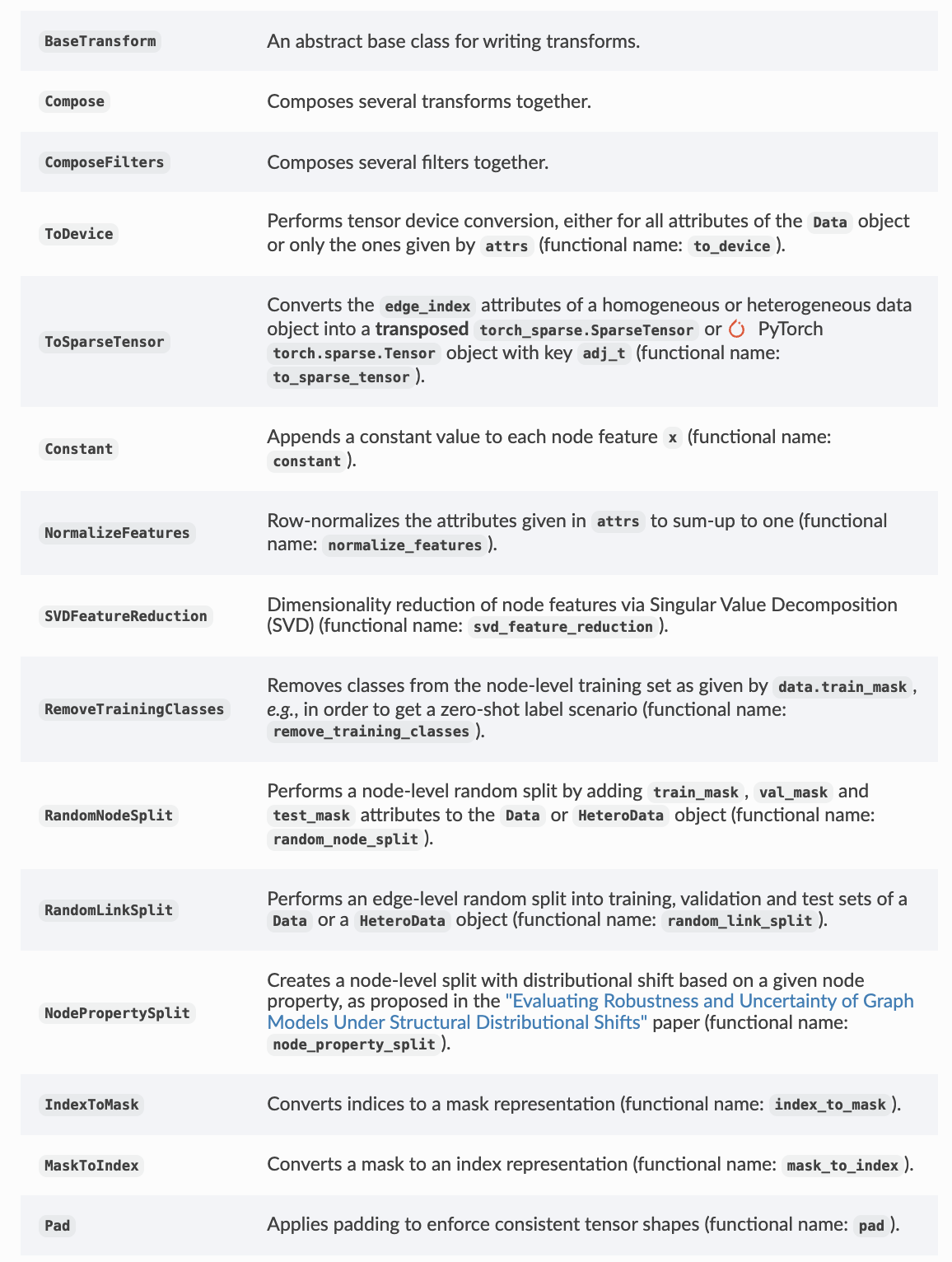
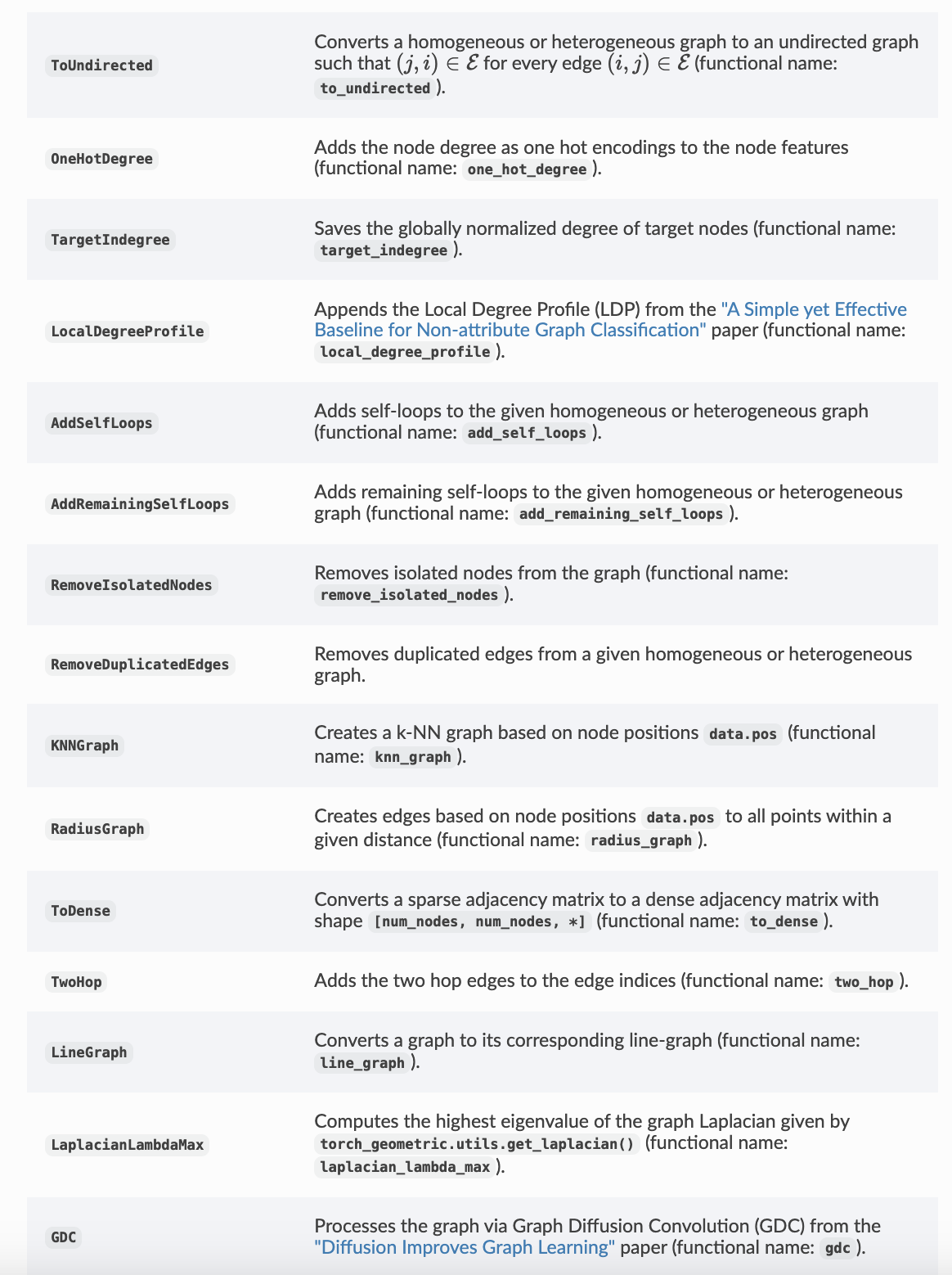
# >>> torch.Size([32, 21])torch_geometric.transforms.Compose to chain transforms.pre_transform) or accessing a graph (transform).For more details, visit the PyTorch Geometric documentation.
For more details, visit the PyTorch Geometric documentation.
Data(x=[2518, 3], y=[2518], pos=[2518, 3], category=[1])We can convert the point cloud dataset into a graph dataset by generating nearest neighbor graphs from the point clouds via transforms:
Data(x=[2518, 3], y=[2518], pos=[2518, 3], category=[1])We use the pre_transform to convert the data before saving it to disk (leading to faster loading times). Note that the next time the dataset is initialized it will already contain graph edges, even if you do not pass any transform. If the pre_transform does not match with the one from the already processed dataset, you will be given a warning.
In addition, we can use the transform argument to randomly augment a Data object, e.g., translating each node position by a small number:
Data(x=[2518, 3], y=[2518], pos=[2518, 3], category=[1])---------- Data Set Properties ----------
type : <class 'torch_geometric.datasets.planetoid.Planetoid'>
Number of graphs : 1
Number of nodal features : 1433
Number of edge features : 0
Number of labels (y) : 2708
Number of classes : 7
---------- Misc Graph Properties ----------
------------------
type : <class 'torch_geometric.data.data.Data'>
shapes: Data(x=[2708, 1433], edge_index=[2, 10556], y=[2708], train_mask=[2708], val_mask=[2708], test_mask=[2708])
Number of nodes : 2708
Number of edges : 10556
x matrix size:
torch.Size([2708, 1433])
y label : tensor(3)
Edge List size:
torch.Size([2, 10556])\[ \mathbf{x}_v^{(\ell + 1)} = \mathbf{W}^{(\ell + 1)} \sum_{w \in \mathcal{N}(v) \, \cup \, \{ v \}} \frac{1}{c_{w,v}} \cdot \mathbf{x}_w^{(\ell)} \]
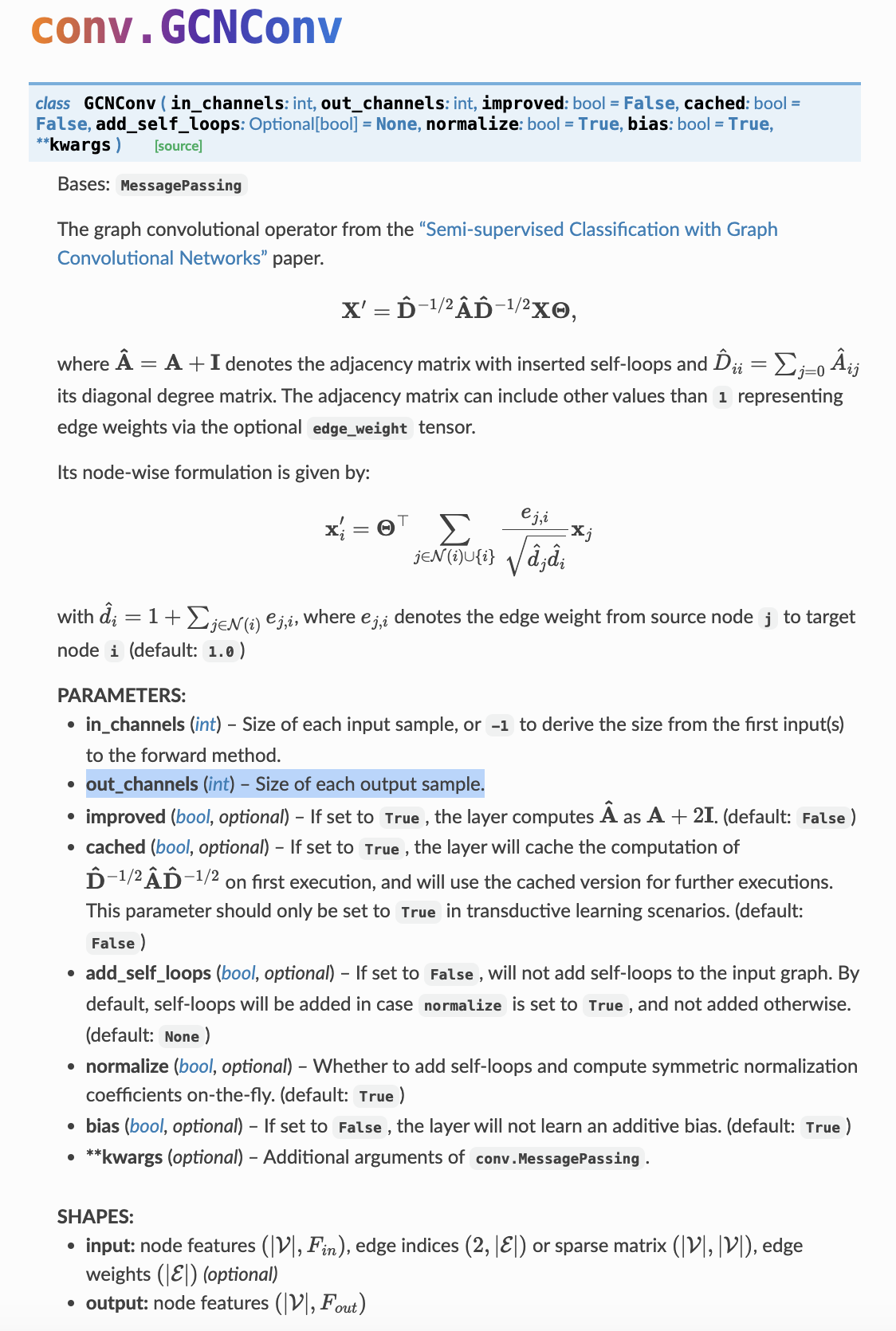
[num_output_features, num_input_features]GCNConv, which can be executed by passing in the node feature representation x and the COO graph connectivity representation edge_index.With this, we are ready to create our
torch.nn.Module class:import torch
import torch.nn.functional as F
from torch_geometric.nn import GCNConv
class GCN(torch.nn.Module):
def __init__(self):
super().__init__()
self.conv1 = GCNConv(dataset.num_node_features, 16)
self.conv2 = GCNConv(16, dataset.num_classes)
def forward(self, data):
x, edge_index = data.x, data.edge_index
x = self.conv1(x, edge_index)
x = F.relu(x)
x = F.dropout(x, training=self.training)
x = self.conv2(x, edge_index)
return F.log_softmax(x, dim=1)device = torch.device('cuda' if torch.cuda.is_available() else 'cpu')
model = GCN().to(device)
data = dataset[0].to(device)
optimizer = torch.optim.Adam(model.parameters(), lr=0.01, weight_decay=5e-4)
print(data.train_mask)
print(sum(data.train_mask==True)/2708)
model.train()
for epoch in range(200):
optimizer.zero_grad()
out = model(data)
# Compute the negative log likelihood loss.
loss = F.nll_loss(out[data.train_mask], data.y[data.train_mask])
loss.backward()
optimizer.step()tensor([ True, True, True, ..., False, False, False])
tensor(0.0517)
tensor(0.3693)Finally, we can evaluate our model on the test nodes: