Spectral clustering and Spectral community detection
What makes a method spectral?
A method is spectral if it derives its answer from the eigenvalues and/or eigenvectors of a matrix built from the data: rather than operating on the raw data points/graph directly.
The pattern:
Build a matrix that encodes structure (\(W\), \(L\), \(B\), adjacency, etc.)
Compute its spectrum (eigenvalues + eigenvectors)
Use the eigenvectors as the answer: either as new coordinates to embed/cluster in, or as a direct signal (e.g., sign → group membership)
What makes a method “spectral” is using eigendecomposition—not the specific matrix or clustering method. All these methods rely on eigenvectors to reveal structure.
Graph Laplacian
Quick review
The Graph Laplacian
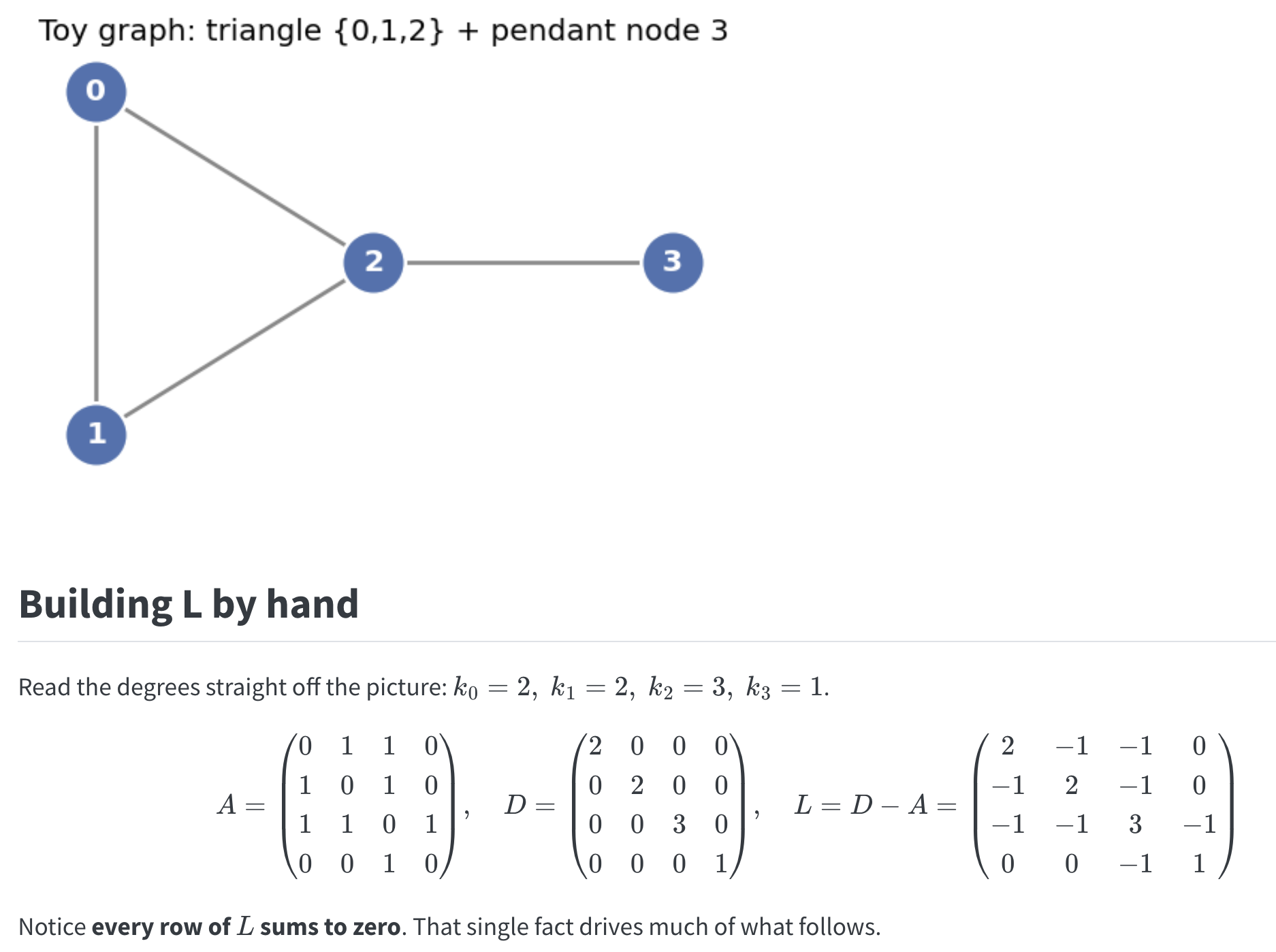
For an undirected, unweighted graph with adjacency matrix \(A\) and degree matrix \(D=\operatorname{diag}\left(k_1, \ldots, k_N\right)\) (degrees on the diagonal, zeros elsewhere):
\[
L=D-A
\]
Diagonal entry \(L_{i i}=k_i\) (the degree of node \(i\) ).
Off-diagonal entry \(L_{i j}=-A_{i j}\) (a -1 wherever an edge exists).
Like \(A\), it is a square matrix that encodes the whole graph, but it carries far more usable spectral structure.
Example:
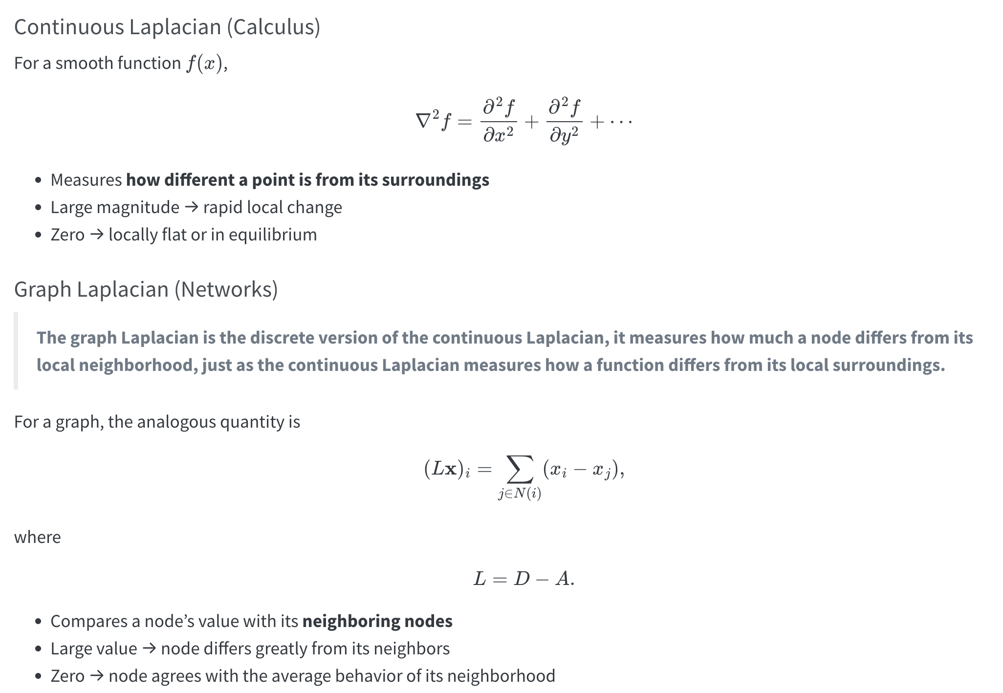
Moving from the Continuous Laplacian to the Graph Laplacian
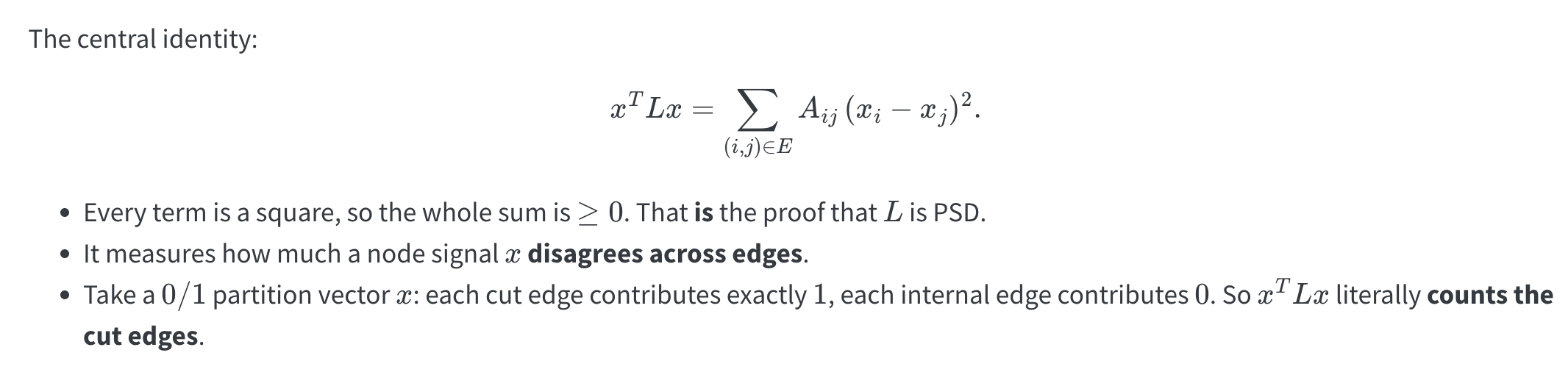
The Quadratic Form
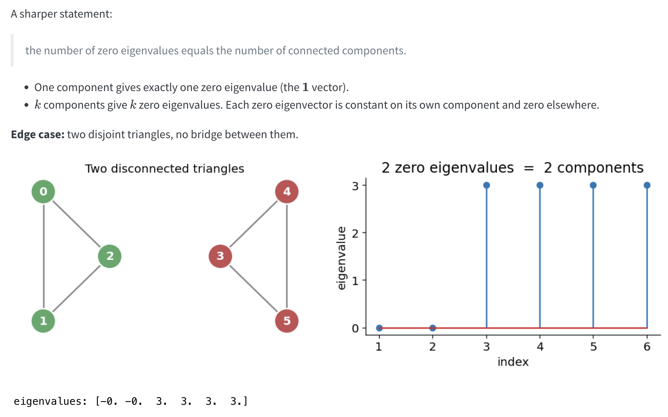
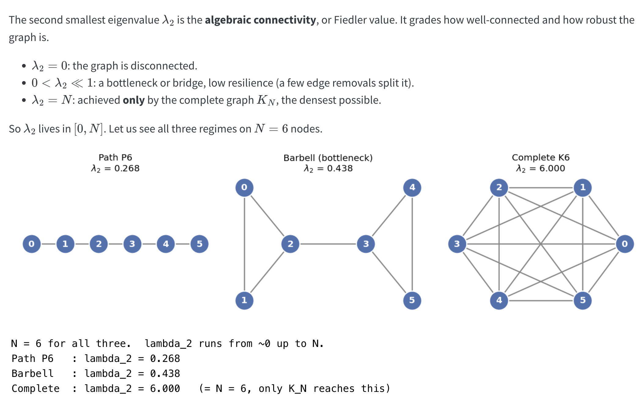
Multiplicity of 0 Counts Components
Algebraic Connectivity: the Fiedler Value
What Does \(L\) Actually Measure?
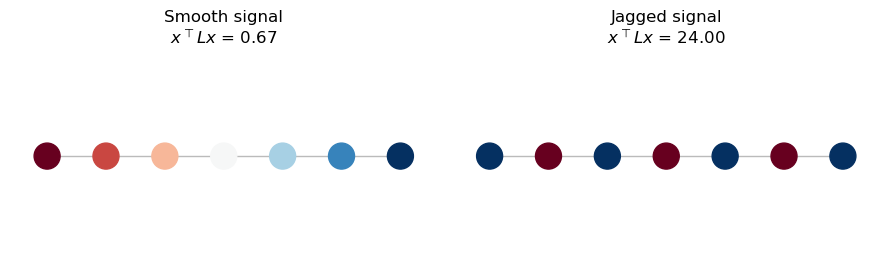
Assign every node a number \(x_i\). The Laplacian measures how much neighbors disagree:
\[
x^\top L x = \tfrac{1}{2}\sum_{(i,j)\in E}(x_i - x_j)^2
\]
Small value → connected nodes have similar values (smooth)
Large value → connected nodes clash
The Laplacian rewards signals that stay smooth along edges: exactly what a community-indicator should do.
Spectral clustering doesn’t cluster the graph directly: it first re-coordinates the nodes.
Take the \(d\) smallest non-trivial eigenvectors of the graph Laplacian \(L\) and stack them as columns. Each row is now a node, described by \(d\) numbers:
\[\text{node } i \;\longmapsto\; \big(v_1(i),\, v_2(i),\, \dots,\, v_d(i)\big) \in \mathbb{R}^d\]
In this space, well-connected nodes land close together and weakly-connected ones drift apart: so communities that were tangled in the raw graph become compact, separable blobs. Ordinary k-means then finishes the job.
Analogy to PCA:
PCA
Spectral embedding
Operates on
covariance matrix
graph Laplacian \(L\)
Keeps
eigenvectors of largest eigenvalues
eigenvectors of smallest (non-zero) eigenvalues
Each axis captures
directions of most variance
directions of smoothest variation over the graph
Payoff
fewer coordinates, most information kept
fewer coordinates, community structure exposed
One line: both replace the original features with a handful of eigenvector coordinates: PCA keeps the axes of greatest spread, spectral clustering keeps the axes of least connective “energy,” where the low end of the Laplacian spectrum is exactly where cluster structure lives.
An intuitive analogy: Laplacians and spring systems
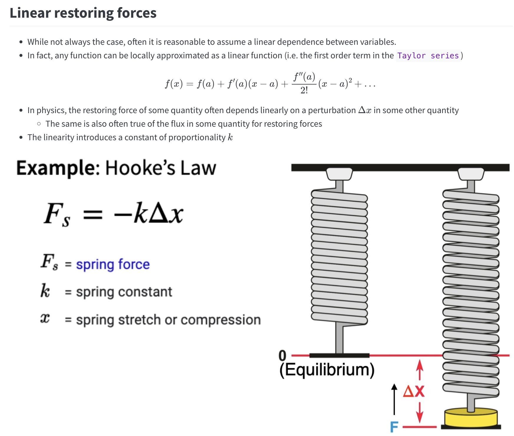
Recall spring system
Warm-up: Two Masses, One Spring
The smallest possible “network”: two nodes, one edge.
where \(u_1\) and \(u_2\) are the displacements \(\Delta x_1\) and \(\Delta x_2\) from equilibrium. \[
K = k\begin{pmatrix}1 & -1\\ -1 & 1\end{pmatrix} = k\,(D-A) = k\,L
\]
The stiffness matrix is the graph Laplacian (times \(k\)). Its two modes:
mode
shape
\(\lambda\)
meaning
drift
\((1,1)\)
\(0\)
both slide together: no spring stretched
stretch
\((1,-1)\)
\(2k\)
masses move apart: the one real oscillation
Note
Takeaway: the spring’s energy \(U=\tfrac{k}{2}(u_1-u_2)^2\) is exactly the Laplacian roughness form. The zero mode is the constant vector: free drift with no restoring force.
A Network Is a Spring Mesh
Now every node is a mass, every edge a spring. The force on node \(i\) just sums its springs:
Look for things that oscillate, \(x(t)=v\,e^{i\omega t}\):
\[
Lv = \omega^2 v
\]
Note
Takeaway: the graph’s normal modes = eigenvectors of \(L\), and each mode’s frequency² = its eigenvalue. Since \(L\succeq 0\), all \(\omega\) are real. “How can this network vibrate?” and “what’s the spectrum of \(L\)?” are the same question.
Takeaway:\(L\)is the discrete \(-\nabla^2\), so the eigenvalue problem \(Lv=\lambda v\) is literally “find the standing waves of the network.” Small \(\lambda\) = low pitch = smooth mode; the sign pattern of each mode is its nodal set: which is why the low modes draw the communities.
Spectral community detection
The Goal: Find the Groups
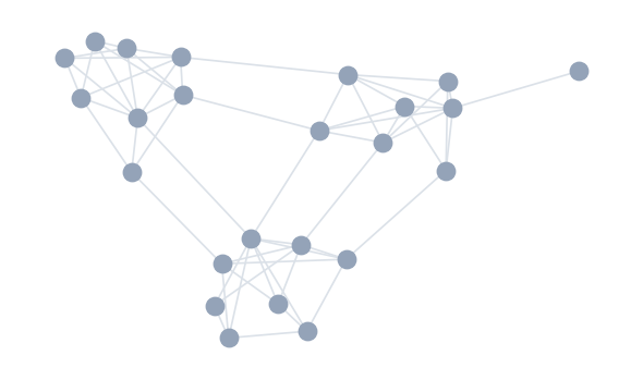
A network often has communities: groups of nodes that are:
Densely connected inside the group
Sparsely connected between groups
Note
The eye spots this instantly. Spectral methods let a machine find it using linear algebra: no guessing at group boundaries.
The Core Idea
Imagine every edge is a spring pulling its two nodes together.
Nodes in the same community are held tightly by many springs
The few springs between communities are the weak links
Spectral clustering asks: if we let this spring system settle into its natural “modes of vibration,” which nodes move together?
Nodes that swing together → same community. -The math that captures this vibration is the graph Laplacian.
Spectral Clustering ≠ Spectral Community Detection
Spectral clustering: a method
Build similarity graph from data → Laplacian eigenvectors → embed → k-means
Input can be any data (point clouds, features)
Spectral community detection: a task on graphs
Find communities in a network that is already a graph
Spectral clustering is one way to do it
The overlap
Run spectral clustering on a network → it is a community detection method
Broader on each side
Clustering → also handles non-network data
Detection → also uses other operators, not just the Laplacian: - Modularity matrix \(B = A - k_ik_j/2m\) (Newman) - Non-backtracking (Hashimoto), Bethe Hessian
Note
Both the Laplacian route and the modularity route are spectral methods for the same task (community detection on a graph).
The Spectrum Reveals Structure
Eigen-decompose \(L\). Its smallest eigenvalues/eigenvectors carry the community signal.
Two key facts:
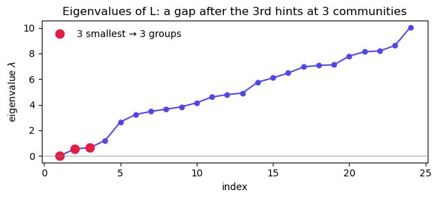
Eigenvalue 0 always exists; its multiplicity = number of connected components
The second-smallest eigenvalue \(\lambda_2\) (the Fiedler value, or algebraic connectivity) is small when the graph is near-splittable
Code
Example: 2 Communities
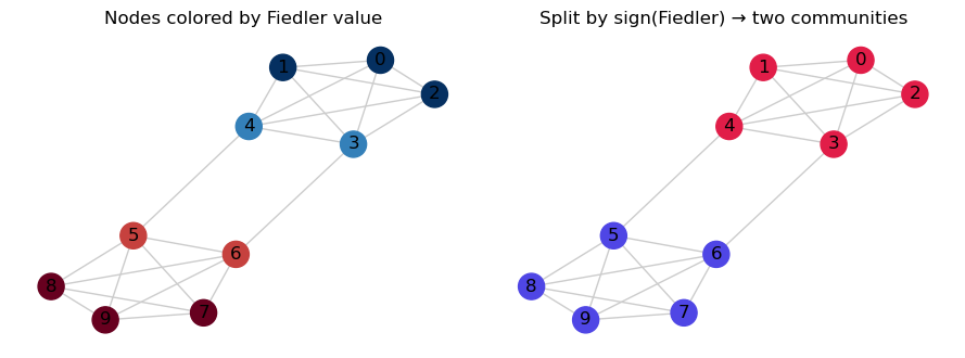
Recall the Fiedler value is the second-smallest eigenvalue of the Laplacian, and its corresponding eigenvector (the Fiedler vector) reveals how the graph can be partitioned into two nearly-disconnected communities.
With two communities, the single Fielder eigenvector (the one tied to the second-smallest Laplacian eigenvalue) assigns each node a real value whose sign: positive versus negative: cleanly splits the graph into its two groups, so you just threshold at zero rather than running k-means.
The General Algorithm (\(k\) communities)
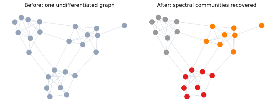
With multiple groups, you simply keep additional eigenvectors, and each node’s values across them become its coordinates in a new feature space; these eigenvector-based embeddings turn every node into a point, and k-means clusters those points into communities.
When you want more than two groups, use \(k\) eigenvectors as coordinates, then cluster:
Build \(L = D - A\)
Compute the \(k\) eigenvectors with smallest eigenvalues
Stack them → each node becomes a point in \(\mathbb{R}^k\) (the spectral embedding)
Run k-means on those points
k-means labels = community assignments
Tip
The spectral step does the hard work: it reshapes a tangled graph into tidy blobs. k-means then does the easy work of separating blobs.
The Fiedler Vector Splits the Graph
For a 2-way split, the eigenvector of \(\lambda_2\) (the Fiedler vector) acts as a soft membership score. Its sign is the answer.
Toy Example: End to End in NetworkX
Code
import networkx as nx, numpy as npfrom sklearn.cluster import KMeans# 1. A graph with three planted communitiesG = nx.stochastic_block_model( [8, 8, 8], [[0.7, 0.04, 0.04], [0.04, 0.7, 0.04], [0.04, 0.04, 0.7]], seed=1)# 2. LaplacianA = nx.to_numpy_array(G)L = np.diag(A.sum(axis=1)) - A# 3. Smallest-k eigenvectors → spectral embeddingk =3vals, vecs = np.linalg.eigh(L)embedding = vecs[:, :k]# 4. k-means on the embeddinglabels = KMeans(n_clusters=k, n_init=10, random_state=0).fit_predict(embedding)
Some clusters are obvious to the eye but invisible to k-means.
Think of two interlocking crescents: clearly two groups, but
k-means fails: it only knows distance to a center, not shape.
The trick: cluster by connectivity, not distance
Build a graph Connect each point to its nearest neighbors. “Same cluster” now means well-connected, not nearby.
Find new coordinates: Take the smallest eigenvectors of the graph Laplacian. → a new space where connected groups pull apart.
Spectral clustering casts the data into a low-dimensional spectral embedding: a space whose coordinates are the leading eigenvectors of the graph’s (Laplacian or adjacency) matrix: where community structure that was tangled in the original graph becomes near-linearly separable, so that geometrically simple clustering (e.g., k-means) suffices.
The shapes become blobs: The tangled crescents map to two clean, separated clumps.
Run k-means: In the embedding, the groups are trivially separable.
Tip
One line:reshape the data using its graph structure, so hard shapes become easy blobs: then cluster the easy way (k-means).
The RBF (Gaussian) Similarity Kernel
Turns distance (usually Euclidean) into similarity: the key building block of the affinity matrix \(W\).
where \(\|\cdot\|_2\) is Euclidean distance. This is what sklearn.metrics.pairwise.rbf_kernel uses by default, and it’s the near-universal convention
Other distance/dissimilarity metrics people substitute in:
Manhattan (L1) - more robust to outliers, sometimes used on high-dimensional sparse data
Mahalanobis distance - accounts for feature correlations/scale: \(\sqrt{\left(x_i-x_j\right)^T \Sigma^{-1}\left(x_i-x_j\right)}\); useful when features aren’t naturally on the same scale
Cosine distance \((1-\cos \theta)\) - common for text/embeddings where direction matters more than magnitude
Geodesic/graph distance - e.g., shortest-path distance on a manifold or existing graph, used in manifold learning (Isomap-style) variants
Custom domain-specific distances - e.g., edit distance for strings, dynamic time warping for time series
once you swap in a non-Euclidean distance, you lose the strict mathematical guarantee that the resulting matrix is a valid positive semi-definite kernel
Intuition in 1D: Similarity vs. Distance
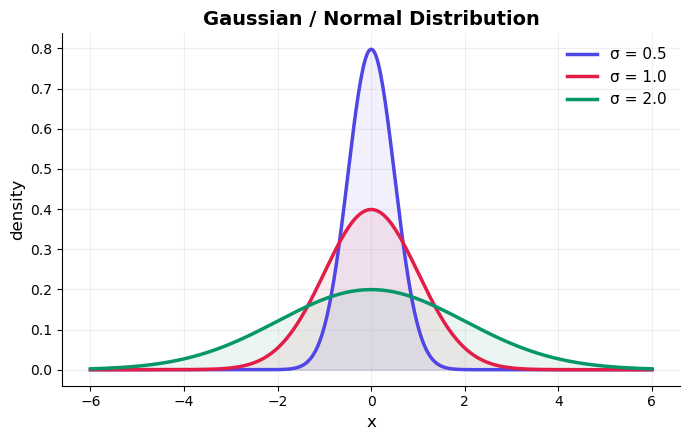
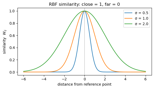
Smaller \(\sigma\) → similarity drops off fast (only very close points count)
Larger \(\sigma\) → similarity stays high over longer distances
Code
import numpy as npimport matplotlib.pyplot as pltdef rbf(d, sigma=1.0):return np.exp(-d**2/ (2* sigma**2))# a fixed point at 0, compare against a range of distancesdistances = np.linspace(-6, 6, 200)plt.figure(figsize=(6, 3.5))for sigma in [0.5, 1.0, 2.0]: plt.plot(distances, rbf(distances, sigma), label=f"σ = {sigma}")plt.axvline(0, color="gray", lw=0.5)plt.xlabel("distance from reference point")plt.ylabel("similarity $W_{ij}$")plt.title("RBF similarity: close = 1, far = 0")plt.legend()plt.tight_layout()plt.show()
From 1D Points to a Similarity Matrix
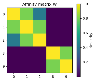
Five points on a line → every pair gets a similarity score → the affinity matrix \(W\).
Notice the block structure: {0,1,2} are mutually similar, {8,9} are mutually similar, and the two blocks are near-zero to each other
That block structure is exactly what the Laplacian eigenvectors will pick up on