Clustering

J. Hickman

Cluster data

Where does clustered data come from?

Cluster generating functions

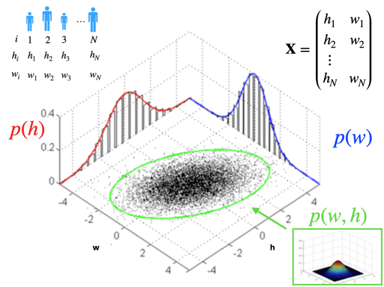
  • Data that forms into groups (i.e. clusters) in some feature space \(\mathbf X\) is typically the result of some data generating process.

  • Process is governed by some data generating probability density function (PDF) \(P(\mathbf X)\)

  • For example, consider a 2D feature space \(\mathbf x = (x_1, x_2)\).

    • In this space different cluster distributions arise by sampling data from different generating PDFs \[ C_1 \rightarrow P_1(x_1,x_2) \,\, , \,\,\ C_2 \rightarrow P_2(x_1,x_2) \,\, , \,\,\ \dots etc\]

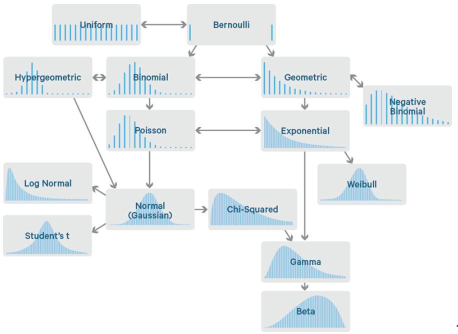
Common single-variable distributions

Examples of various common probability density functions

Single variable Gaussian

  • One of the most common probability distributions is the normal distribution
    • AKA the bell curve or normal distribution
  • If there is only one feature \(x\), then the Normal distribution PDF takes the following form \[ f(x)={\frac {1}{\sigma {\sqrt {2\pi }}}}e^{-{\frac {1}{2}}\left({\frac {x-\mu }{\sigma }}\right)^{2}} \leftarrow \text{two parameters: } \,\, (\mu, \sigma) \]
  • Normally distributed clusters: In many cases, clustering data arise from sampling from a normal distributions

Code: Single variable Gaussian

Code
import numpy as np
import seaborn as sns
import pandas as pd 
import matplotlib.pyplot as plt

# sns.set(rc={'figure.figsize':(11.7,8.27)})

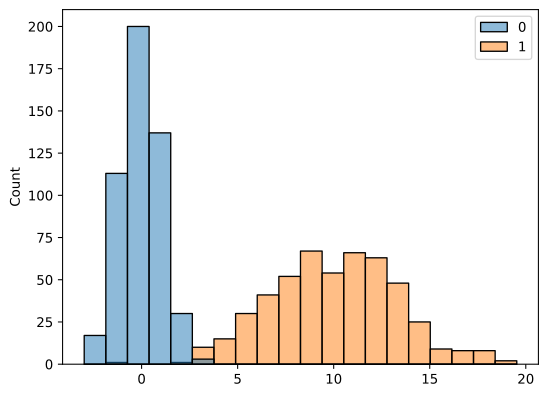
N=500
C1=np.random.normal(loc=0.0, scale=1.0, size=(N,1))
C2=np.random.normal(loc=10.0, scale=3.0, size=(N,1))

sns.histplot(pd.DataFrame(np.hstack((C1,C2))),bins=20)
plt.show()

Figure 1: The plot shows distinct groupings of data exhibiting bimodality due to the sampling from two different generating functions

Two-variable normal distribution

  • The normal distribution can be generalized to higher dimensional features spaces

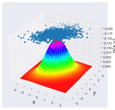
  • In two-dimensions the Gaussian function becomes \[ f(x,y)={\frac {1}{2\pi \sigma _{X}\sigma _{Y}{\sqrt {1-\rho ^{2}}}}}\mathrm {e} ^{-{\frac {1}{2(1-\rho ^{2})}}\left[({\frac {x-\mu _{X}}{\sigma _{X}}})^{2}-2\rho ({\frac {x-\mu _{X}}{\sigma _{X}}})({\frac {y-\mu _{Y}}{\sigma _{Y}}})+({\frac {y-\mu _{Y}}{\sigma _{Y}}})^{2}\right]}\]

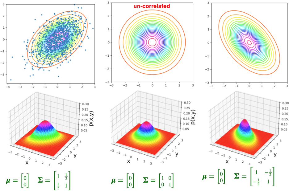
  • Where \(\rho_{x,y}=\frac {\operatorname {cov} (x,y)}{\sigma _{x}\sigma _{y}}\) is the Pearson correlation coefficient

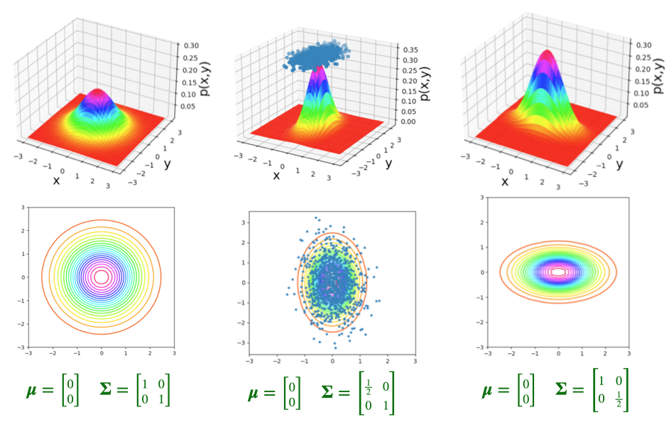
  • The function parameters are \(\mathbf{\mu} =\begin{pmatrix}\mu _{X} \\ \mu _{Y}\end{pmatrix}\) and \({\boldsymbol \Sigma }=\begin{pmatrix}\sigma _{X}^{2}&\rho \sigma _{X}\sigma _{Y}\\\rho \sigma _{X}\sigma _{Y}&\sigma _{Y}^{2}\end{pmatrix}\)

Visualization

  • The following image shows a graphical representation of this concept

Parameterizations: Un-correlated

Example of various parametrizations of the un-correlated two-variable Gaussian distribution

Parameterizations: Correlated

Example of various parametrizations of the correlated two-variable Gaussian distribution

Code: Two-variable Gaussian-1

Code
# Source: The code was modified from https://www.geeksforgeeks.org/visualizing-the-bivariate-gaussian-distribution-in-python/


# Importing the necessary modules
import numpy as np
import matplotlib.pyplot as plt
from scipy.stats import multivariate_normal
 
plt.style.use('seaborn-dark')
plt.rcParams['figure.figsize']=14,6
 
# Initializing the random seed
random_seed=1000
 
# List containing the variance
# covariance values
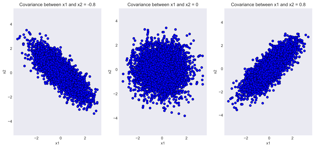
cov_val = [-0.8, 0, 0.8]
 
# Setting mean of the distributino to
# be at (0,0)
mean = np.array([0,0])
 
# Iterating over different covariance
# values
for idx, val in enumerate(cov_val):
    plt.subplot(1,3,idx+1)
     
    # Initializing the covariance matrix
    cov = np.array([[1, val], [val, 1]])
     
    # Generating a Gaussian bivariate distribution
    # with given mean and covariance matrix
    distr = multivariate_normal(cov = cov, mean = mean,
                                seed = random_seed)
     
    # Generating 5000 samples out of the
    # distribution
    data = distr.rvs(size = 5000)
     
    # Plotting the generated samples
    plt.plot(data[:,0],data[:,1], 'o', c='blue',
             markeredgewidth = 0.5,
             markeredgecolor = 'black')
    plt.title(f'Covariance between x1 and x2 = {val}')
    plt.xlabel('x1')
    plt.ylabel('x2')
    plt.axis('equal')
     
plt.show()

anti-correlated, un-correlated, positively correlated normally distributed data

Code: Two-variable Gaussian-2

Code
import matplotlib.pyplot as plt
import numpy as np

#USER INPUTS
FUNC=2
FS=18   #FONT SIZE
CMAP='hsv' #'RdYlBu'

#normal distribution param
ux=0.0; uy=0.0
sx=1.0; sy=1.0                              #STD-DEV
rho=0.5;                                    #[0,1) RHO=PEARSON CORRELATION
u=np.array([[ux],[uy]])                     #MEAN VECTOR u=[ux,uy] 
s=np.array([[sx**2.0,rho*sy*sx],[rho*sy*sx,sy**2.0]])   #COVARIANCE METRIC

#GENERATE POINTS SAMPLED FROM DISTRIBUTION
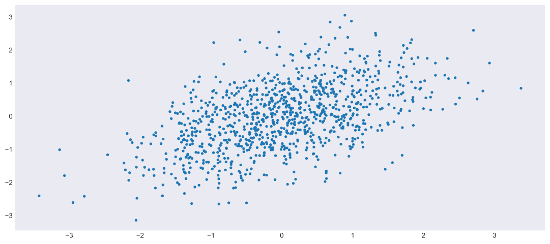
xp, yp = np.random.multivariate_normal(u.reshape(2), s, 1000).T

# DEFINE FUNCTION 
def N(x, y):
    out=1.0/(2*3.1415*sx*sy*(1-rho**2.0)**0.5)
    out=out*np.exp(-(((x-ux)/sx)**2.0-2*rho*((x-ux)/sx)*((y-uy)/sy)+((y-uy)/sy)**2.0)/(2*(1-rho**2)))
    return out

#MESH-1 (SMALLER)
L=3*max(sx,sy)
xmin=-L; xmax=L; ymin=-L; ymax=L
x,y = np.meshgrid(np.linspace(xmin,xmax,20),np.linspace(ymin,ymax,20))

#MESH-2 (DENSER)
X, Y = np.meshgrid(np.linspace(xmin, xmax, 40), np.linspace(ymin, ymax, 40))

#SURFACE PLOT 
fig, ax = plt.subplots(subplot_kw={"projection": "3d"})
ax.set_xlabel('x', fontsize=FS); ax.set_ylabel('y', fontsize=FS); ax.set_zlabel('p(x,y)', fontsize=FS)
surf=ax.plot_surface(X, Y, N(X, Y), cmap=CMAP) 
ax.scatter(xp, yp, 1.1*np.max(N(X, Y)) , '.')
plt.show(); 

Visualization

Code
#SCATTER PLOT
plt.plot(xp, yp,'.')
plt.show(); 

Visualization

Code
#CONTOUR PLOT 
# plt.axis('equal')
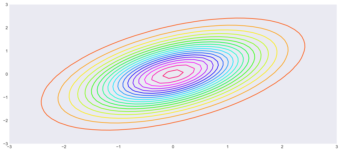
plt.contour(X, Y, N(X, Y), 20, cmap=CMAP); 
plt.show(); 

Code: Cluster-data-generation

Code
#-------------------------------
#GENERATE DATA AND LABELS 
#-------------------------------
import matplotlib.pyplot as plt
import numpy as np
import json 

#DATA GENERATION PARAMETERS 
NUM_CLUSTERS_TO_MAKE=3

sets={}
#GENERATE CLUSTERS FROM 2D NORMAL DISTANCE
for cluster in range(0,NUM_CLUSTERS_TO_MAKE):
    NPOINTS=int(np.random.uniform(low=100, high=300, size=1))

    #normal distribution param
    L=5
    ux=np.random.uniform(-L,L,size=1)[0]; 
    uy=np.random.uniform(-L,L,size=1)[0];
    sx=np.random.uniform(0.25*L,0.75*L,size=1)[0]; 
    sy=np.random.uniform(0.25*L,0.75*L,size=1)[0];          #STD-DEV
    rho=np.random.uniform(0.0,.99,size=1)[0];       #[0,1) RHO=PEARSON CORRELATION
    u=np.array([ux,uy])
    S=np.array([[sx**2.0,rho*sy*sx],[rho*sy*sx,sy**2.0]])   #COVARIANCE METRIC

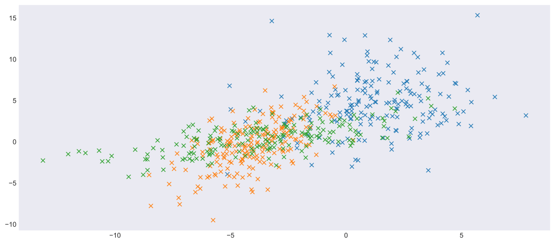
    x, y = np.random.multivariate_normal(u, S, NPOINTS).T
    plt.plot(x, y, 'x')
    sets[cluster]=[x.tolist(),y.tolist()]
    # plt.axis('equal')
plt.show()

with open('01-cluster_data.json', 'w', encoding='utf-8') as f:
    json.dump(sets, f, indent=4)

Multi-variable normal distribution

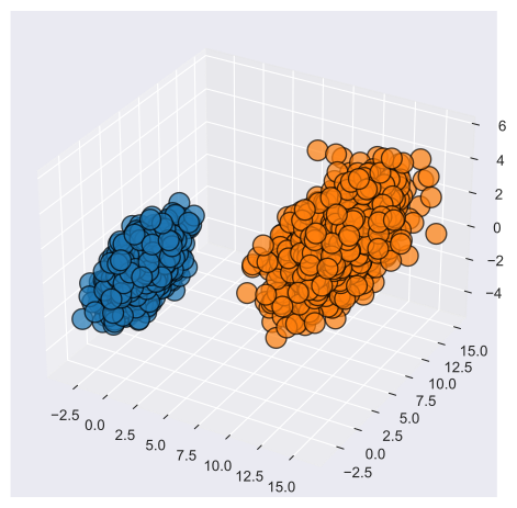
  • Normal distribution can be generalized to arbitrarily high dimensional features space

  • In N-dimensions the Gaussian function becomes \[ {\displaystyle f_{\mathbf {X} }(x_{1},\ldots ,x_{k})={\frac {\exp \left(-{\frac {1}{2}}({\mathbf {x} }-{\boldsymbol {\mu }})^{\mathrm {T} }{\boldsymbol {\Sigma }}^{-1}({\mathbf {x} }-{\boldsymbol {\mu }})\right)}{\sqrt {(2\pi )^{k}|{\boldsymbol {\Sigma }}|}}}}\]

  • Where \(\mathbf{\mu}\) is the vector of means of the data-cloud

  • And \({\boldsymbol \Sigma }\) is the covariance matrix

Code: Three dimensional Gaussian

Code
import matplotlib.pyplot as plt
import numpy as np

#normal distribution param
ux=0.0; uy=0.0; uz=0.0
sx=1.0; sy=1.0; sz=1.0              #STD-DEV
rho=0.5;                            #[0,1) RHO=PEARSON CORRELATION
u1=np.array([[ux],[uy],[uz]])       #MEAN VECTOR u=[ux,uy,uz] 
s=np.array([
 [sx**2.0,rho*sx*sy,rho*sx*sz]
,[rho*sy*sx,sy**2.0,rho*sy*sz]
,[rho*sz*sx,rho*sz*sy,sz**2.0]])    #COVARIANCE METRIC
u2=np.array([[10],[10],[0]])        #MEAN VECTOR u=[ux,uy,uz] 

#GENERATE POINTS SAMPLED FROM DISTRIBUTION
x1, y1, z1= np.random.multivariate_normal(u1.reshape(3), s, 1000).T
x2, y2, z2= np.random.multivariate_normal(u2.reshape(3), 3*s, 1000).T

#SCATTER PLOT
fig = plt.figure(figsize=(6, 6))
ax = fig.add_subplot(111, projection='3d')
ax.scatter(x1, y1, z1,
           linewidths=1, alpha=.7,
           edgecolor='k',
           s = 200,
           )
ax.scatter(x2, y2, z2,
           linewidths=1, alpha=.7,
           edgecolor='k',
           s = 200,
           )
plt.show()

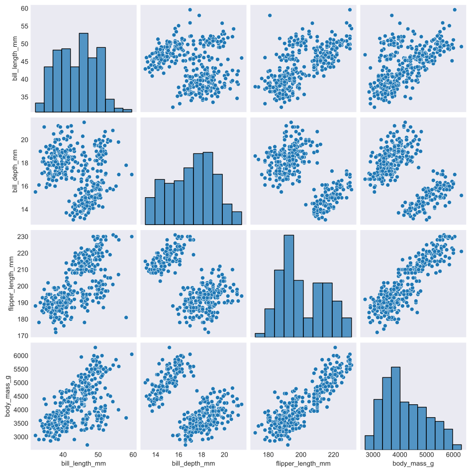
Code: Penguins-1

Code
import seaborn as sns
import matplotlib.pyplot as plt

penguins = sns.load_dataset("penguins")

sns.pairplot(penguins)
plt.show()
Code
# print(penguins.describe())

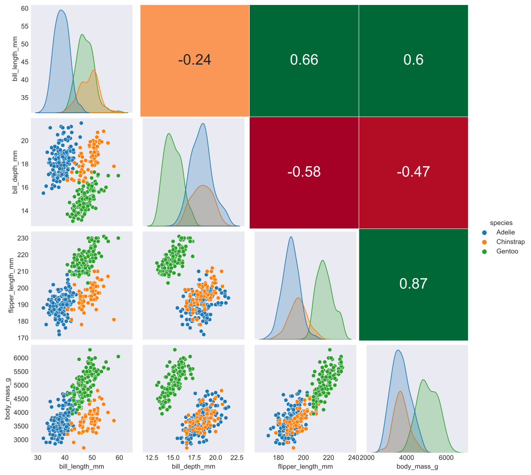
Code: Penguins-2

Code
import numpy as np
import pandas as pd
import seaborn as sns
import matplotlib.pyplot as plt

def hide_current_axis(*args, **kwds):
    plt.gca().set_visible(False)

d1 = penguins

e = sns.pairplot(d1,hue="species")
e.map_upper(hide_current_axis)

(xmin, _), (_, ymax) = e.axes[0, 0].get_position().get_points()
(_, ymin), (xmax, _) = e.axes[-1, -1].get_position().get_points()

ax = e.fig.add_axes([xmin, ymin, xmax - xmin, ymax - ymin], facecolor='none')

corr1 = d1.corr()
mask1 = np.tril(np.ones_like(corr1, dtype=bool))
sns.heatmap(corr1, mask=mask1, cmap='RdYlGn', vmax=.5, vmin=-.5,
            linewidths=.5, cbar=False, annot=True, annot_kws={'size': 22}, ax=ax)
ax.set_xticks([])
ax.set_yticks([])
# ax.xaxis.tick_top()
# ax.yaxis.tick_right()

plt.show()

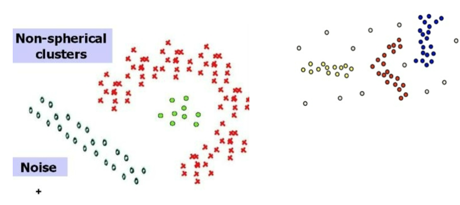
Non-Gaussian clusters

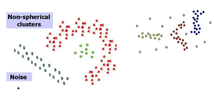
  • It is important to emphasize that NOT all clusters are normally distributed

Source: Introduction to Data Mining (Second Edition) (Vipin Kumar) https://www-users.cse.umn.edu/~kumar001/dmbook/index.php

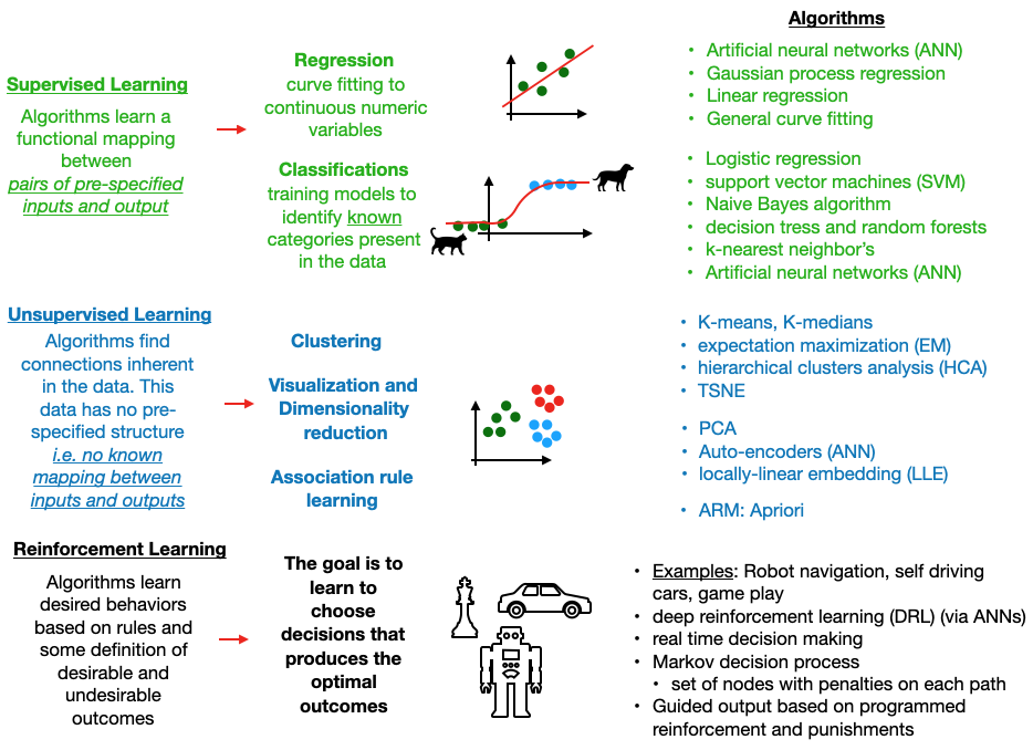
Unsupervised learning

Introduction to Unsupervised machine learning

Supervision

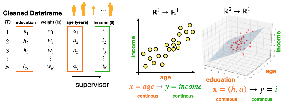
  • Supervised case-1 (regression): A supervisor has identified a relationship in the data between some numerical inputs \(X\) and some numerical targets.
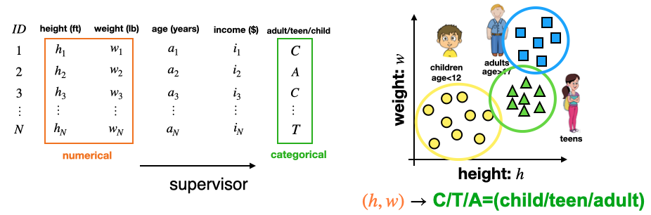
  • Supervised case-2 (classification): A supervisor has isolated a relationship in the data between some Numerical inputs \(X\) and some categorical targets \(y\) (i.e. labels)
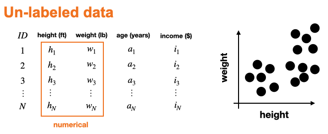
  • Un-supervised case: There are NO KNOWN labels or mappings are present in the data.

Machine learning categories

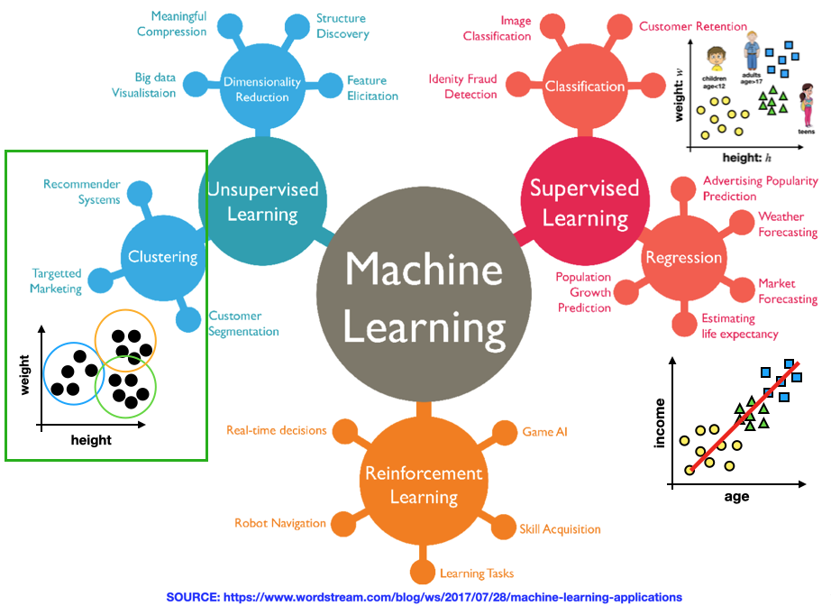
Un-supervised learning:

  • Typically when doing unsupervised learning (i.e. clustering or dimensionality reduction) you DO NOT know if any relevant mappings (relationships) in the data.
  • In this case, there is NO KNOWN “target” space \(Y\) w/ the “ground truth” labels (targets).
  • Instead, you have some features space \(\mathbf X\) and you are trying to systematically figure out if the data in that space forms groups (clusters).
  • This “un-labeled” nature of the data-set is what makes it “unsupervised”.
  • It is possible to already have some categorical labels in your data before clustering. In this case, the clustering algorithm may or may-not find clusters corresponding to the existing labels.
  • If it finds new labels, this suggests that there may be unknown groups in the data which are NOT associated with the existing labels.

ML Algorithms

Clustering

Introduction to clustering analysis

What is clustering?

  • Clustering is an unsupervised learning technique.
    • The data is not labeled or do not specify a given class.
  • Goal:
    • Discover clusters or groups within the data that are similar
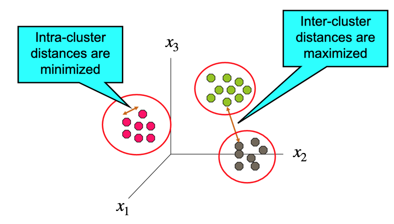
    • Find groups (i.e. clusters), based on some notion of similarity or distance in a feature space \(X\) , such that elements in the same cluster are more similar to each other than they are to elements in different clusters).

Motivation

  • Why Cluster Data?
    • Group related items to reveal internal structure of the data
    • Knowledge discovery during EDA (i.e. pattern identification)
    • Subset selection: Reduce the size of large data sets by considering sub-sets (US –> PA, NY, DC, … etc)
  • Typical Clustering Objectives
    • Find the number of clusters
    • Find the number of points within each cluster
    • Find the distance of objects within each cluster
    • Find the distance between different clusters
    • Find the density of points within a cluster

What is NOT Cluster Analysis?

  • Supervised classification
    • The training data have labels or classes so that the classification method can “learn” how to classify new data into the correct group.
  • Simple segmentation
    • Creating groups based on a feature.
    • Dividing students into different registration groups alphabetically by last name: Group A, Group B, etc…
  • Results of a query
    • Groupings are a result of an external specification – the groups are pre-defined.

What is a cluster?

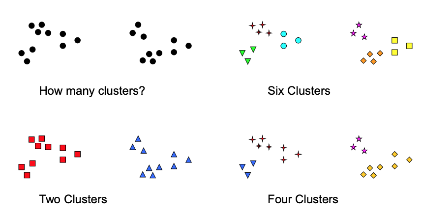
  • This question is ambiguous and subjective & often clusters are not well defined
  • Clustering results require more “scrutiny” than supervised results

Source: Introduction to Data Mining (Second Edition) (Vipin Kumar) https://www-users.cse.umn.edu/~kumar001/dmbook/index.php

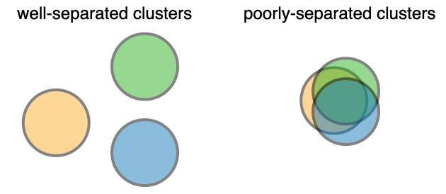
Separation & Exclusivity

  • Separation
  • Exclusivity
    • Exclusive - Assigns each data point to a single cluster
    • Non-exclusive - A data point can be a member of more than one cluster

Search space size

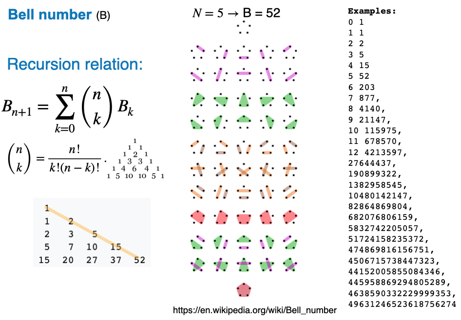
  • The number of possible clusters (increases extremely fast w/ the number of data points)
  • The problem is computationally difficult (NP-hard)

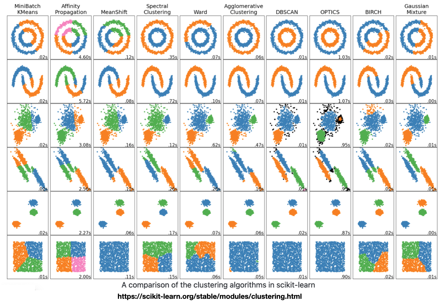
Algorithm result comparison

Hierarchical vs. Partitional

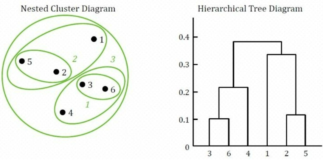
  • An important difference between certain clustering methods is whether the set of clusters are nested or not.
  • Partitional clustering:
    • a division of the set of data into non-overlapping clusters.
    • k means – creates k partitions or clusters
    • Each data point is in exactly one cluster.
  • Hierarchical clustering:
    • nested clustered, organized like a tree.
    • Does not assume a value of k (unlike k-means)

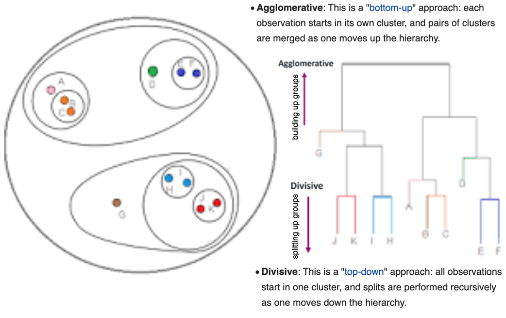
Hierarchical: Agglomerative vs Division

  • Agglomerative (bottom up): Each observation starts in its own cluster, and pairs of clusters are merged as one moves up the hierarchy.
  • Division (top down): All observations start in one cluster, and splits are performed recursively as one moves down the hierarchy.

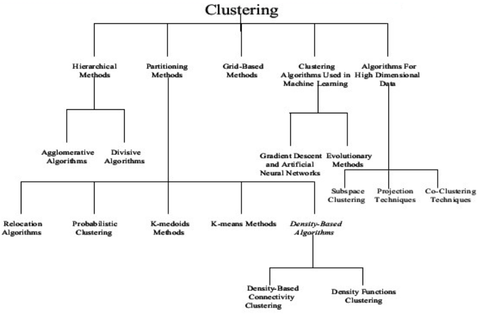
Clustering algorithm summary

K-Means clustering

Introduction:

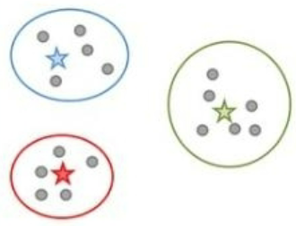
Centroid based cluster identification

  • The center of a cluster is often called a centroid
  • This can be computed using centrality measures associated with the distribution of the data features \(\mathbf x= x_1,x_2 ... x_N\)
    • e.g. (mean, median, or mode)
  • It is helpful to think of the centroid as the most “representative” point of a cluster.
  • You can associate a point to a cluster with the nearest centroid, which is what is done in K-means
  • This is known as Prototype-based clustering
  • A cluster is a set of objects such that an object in a cluster is closer (more similar) to the prototype or “center” of a cluster, than to the center of any other cluster
    Source: Introduction to Data Mining (Second Edition) (Vipin Kumar) https://www-users.cse.umn.edu/~kumar001/dmbook/index.php

Overview

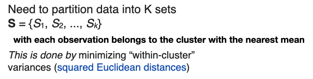
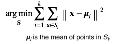
  • k-means clustering is a method of vector quantization, that aims to partition n observations into k clusters in which each observation belongs to the cluster with the nearest mean (cluster centers or cluster centroid)
  • This centroid serves as a prototype of the cluster.
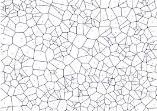
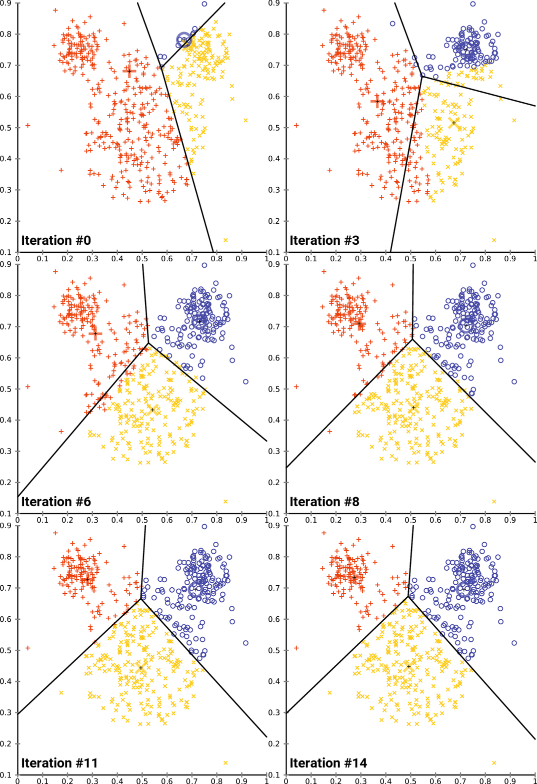
  • This results in a partitioning of the data space into Voronoi cells.
  • K-means clustering minimizes within-cluster variances (squared Euclidean distances), but not regular Euclidean distances,
  • the mean optimizes squared errors, whereas only the geometric median minimizes Euclidean distances.
  • For instance, better Euclidean solutions can be found using k-medians and k-medoids.
    Source: (https://en.wikipedia.org/wiki/K-means_clustering)

Pairwise distances (review)

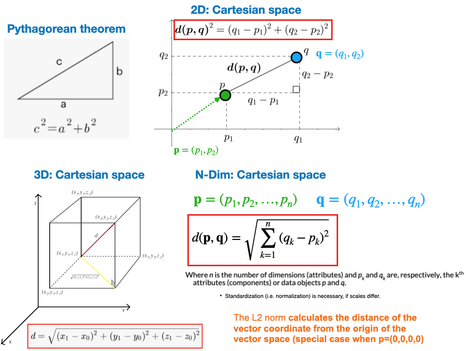
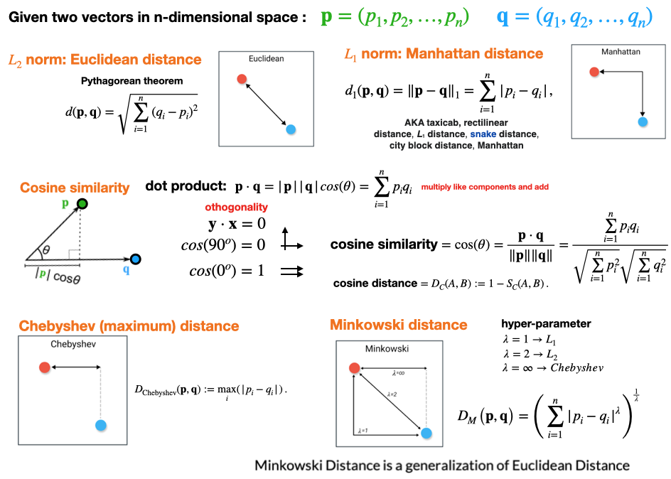
  • Typically, the main ingredient for data clustering is a similarity or difference measure between the data points.
  • L2: Euclidean distance.

Pairwise distances (review)

  • Alternative metrics.

Algorithm

  • The k-means problem is solved using either Lloyd’s or Elkan’s algorithm.
  • In practice, the k-means algorithm is very fast (one of the fastest clustering algorithms available), but it falls in local minima.
    • That’s why it can be useful to restart it several times ## Goal

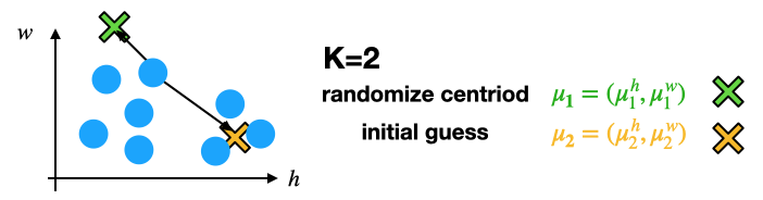
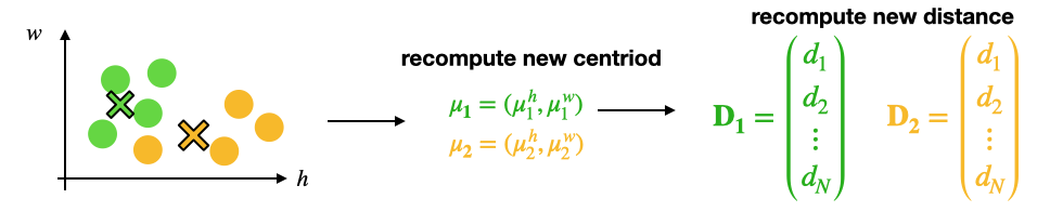
Initialize

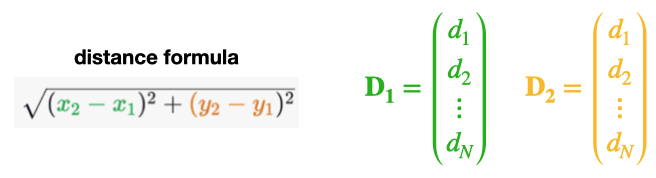
Compute distances to all centroids

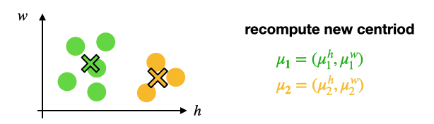
Assign points to nearest centroid and re-compute.

Assign points to nearest centroid and re-compute.

Repeat until converged.

Source: https://en.wikipedia.org/wiki/K-means_clustering

Convergence visualization

Sklearn: cluster.KMeans

  • class sklearn.cluster.KMeans(n_clusters=8, *, init='k-means++', n_init=10, max_iter=300, tol=0.0001, verbose=0, random_state=None, copy_x=True, algorithm='lloyd')
  • Important hyper-parameters
    • n_clusters
      • The number of clusters to form as well as the number of centroids to generate.
    • init
      • Method for initialization:
      • ‘random’: choose n_clusters observations (rows) at random from data for the initial centroids.
      • ‘k-means++’ : selects initial cluster centroids using sampling based on an empirical probability distribution of the points’ contribution to the overall inertia
    • n_init
      • Number of time the k-means algorithm will be run with different centroid seeds.
      • The final results will be the best output of n_init consecutive runs in terms of inertia.
  • https://scikit-learn.org/stable/modules/generated/sklearn.cluster.KMeans.html

DBSCAN

Introduction

Density-based cluster identification

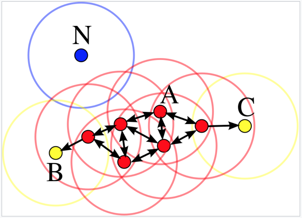
  • A cluster is a dense region of points, which is separated by low density regions, from other regions of high density.
  • Density based methods are particularly useful when the clusters are irregular or intertwined OR when noise and outliers are present.

Overview

  • Density-based spatial clustering of applications with noise (DBSCAN) is a density-based clustering non-parametric algorithm:
  • Given a set of points in some space, it groups together points that are closely packed together (points with many nearby neighbors).

Details

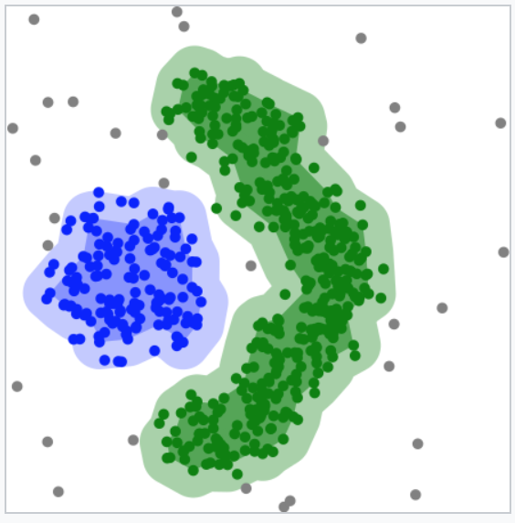
  • Outliers are marked as points that lie alone in low-density regions (whose nearest neighbors are too far away).
  • DBSCAN is one of the most common clustering algorithms and also most cited in scientific literature
  • DBSCAN can find non-linearly separable clusters.
    • This dataset cannot be adequately clustered with k-means clustering.

https://en.wikipedia.org/wiki/DBSCAN

Sklearn: DBSCAN

  • class sklearn.cluster.DBSCAN(eps=0.5, *, min_samples=5, metric='euclidean', metric_params=None, algorithm='auto', leaf_size=30, p=None, n_jobs=None)
  • https://scikit-learn.org/stable/modules/generated/sklearn.cluster.DBSCAN.html
Code
from sklearn.cluster import DBSCAN
import numpy as np
X = np.array([[1, 2], [2, 2], [2, 3],
              [8, 7], [8, 8], [25, 80]])
clustering = DBSCAN(eps=3, min_samples=2).fit(X)
print(clustering.labels_)
print(clustering)
[ 0  0  0  1  1 -1]
DBSCAN(eps=3, min_samples=2)

Hyper-parameter tuning: Clustering

Elbow method: Overview

  • Elbow method is a technique used to determine the optimal number of clusters in a clustering algorithm, typically applied in K-means clustering.

    • Fit the clustering algorithm (e.g., K-means) to the dataset with a range of possible cluster numbers (k).
    • For each value of k, calculate the sum of squared distances (SSD) between data points and their assigned cluster centroids.
    • Plot the SSD values for different k values.
    • Look for an “elbow” point on the plot, where the SSD begins to level off. This is the point where adding more clusters doesn’t significantly reduce the SSD.
    • The number of clusters at the “elbow” point is considered the optimal choice for the problem.
    • It helps strike a balance between model complexity and data fitting.
  • The goal is to find the value of k that represents a meaningful structure in the data without over-segmenting or under-segmenting the dataset.

Elbow method

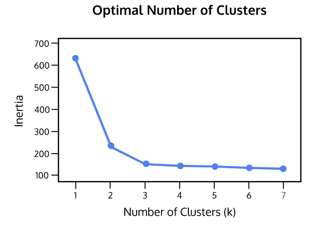
  • Inertia: Sum of squared distances of samples to their closest cluster center
    • weighted by the sample weights if provided
    • This measures how well a dataset was clustered by K-Means.
    • A good model is one with low inertia AND a low number of clusters (K).
    • However, this is a tradeoff because as K increases, inertia decreases.
    • To find the optimal K for a dataset, use the Elbow method; find the point where the decrease in inertia begins to slow.
    • K=3 is the “elbow” of this graph.
      Source: https://www.codecademy.com/learn/machine-learning/modules/dspath-clustering/cheatsheet

Silhouette method

The silhouette method is a technique used to evaluate the quality of clustering in unsupervised learning.

  • For each data point, calculate its silhouette score, which measures how similar it is to its own cluster compared to other clusters.
  • The silhouette score ranges from -1 (poor clustering) to +1 (well-separated clusters). A score near 0 suggests overlapping clusters.
  • Calculate the average silhouette score for all data points in the dataset.
  • Repeat the steps for different numbers of clusters (k) & compare the silhouette scores.
  • Choose the number of clusters (k) that maximizes the average silhouette score.
  • Higher silhouette scores indicate better-defined clusters, making it a useful method for cluster validation and selection.

Silhouette method

  • Silhouette analysis is used to study separation distance between the resulting clusters.
  • The silhouette plot displays a measure of how close each point in one cluster is to points in the neighboring clusters.
  • It provides a way to assess parameters like number of clusters visually.
  • Silhouette coefficients
    • This measure has a range of [-1, 1].
    • +1 indicate that the sample is far away from the neighboring clusters
    • 0 indicates that the sample is on or very close to the decision boundary between two neighboring clusters
    • negative values indicate that those samples may be assigned to the wrong cluster.
      Source: https://www.codecademy.com/learn/machine-learning/modules/dspath-clustering/cheatsheet

Extra

Code examples

Code: Cluster generation function

Code
import numpy as np
import matplotlib.pyplot as plt
import sklearn
Code
def generate_2D_normal_clusters(points_per_cluster=200, num_cluster=3, correlated=True):
    #DATA GENERATION PARAMETERS 

    sets={}
    #GENERATE CLUSTERS FROM 2D NORMAL DISTANCE
    for cluster in range(0,num_cluster):
        # points_per_cluster=int(np.random.uniform(low=100, high=300, size=1))

        #normal distribution param
        L=10
        ux=np.random.uniform(-L,L,size=1)[0]; 
        uy=np.random.uniform(-L,L,size=1)[0];
        sx=np.random.uniform(0.1*L,0.25*L,size=1)[0]; 
        sy=np.random.uniform(0.1*L,0.25*L,size=1)[0];           #STD-DEV
        rho=np.random.uniform(0.0,.99,size=1)[0];       #[0,1) RHO=PEARSON CORRELATION
        u=np.array([ux,uy])
        S=np.array([[sx**2.0,rho*sy*sx],[rho*sy*sx,sy**2.0]])   #COVARIANCE METRIC
        if(correlated==False): 
            S[0,1]=0; S[1,0]=0
        
        x1, x2 = np.random.multivariate_normal(u, S, points_per_cluster).T

        if cluster==0:
            X=np.array([x1,x2]).T
            y=cluster*np.ones(points_per_cluster)
        else: 
            X=np.concatenate((X,np.array([x1,x2]).T),axis=0)
            y=np.concatenate((y,cluster*np.ones(points_per_cluster)),axis=0)

    return X,y

# GENERATE DATA
num_clusters_real=1+int(7*np.random.uniform(0,1))
print(num_clusters_real)
X,y = generate_2D_normal_clusters(points_per_cluster=200, num_cluster=num_clusters_real, correlated=True)
print(X.shape,y.shape)

#FORCE CONTIGUOUS
X=np.ascontiguousarray(X) 
4
(800, 2) (800,)

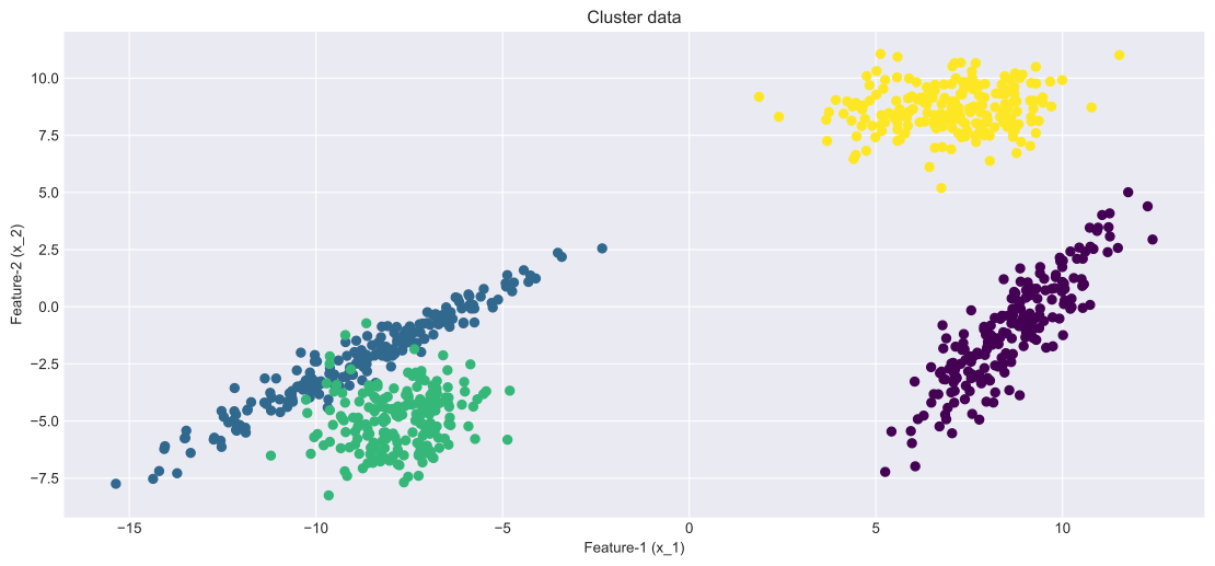
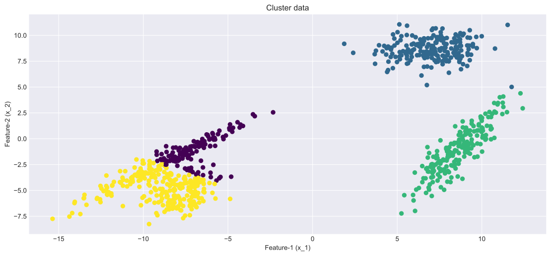
Plot cluster data

Code
# UTILITY PLOTTING FUNCTION
def plot(X,color_vector):
    fig, ax = plt.subplots()
    ax.scatter(X[:,0], X[:,1],c=color_vector, cmap="viridis") #, alpha=0.5) #, c=y
    ax.set(xlabel='Feature-1 (x_1)', ylabel='Feature-2 (x_2)',
    title='Cluster data')
    ax.grid()
    # fig.savefig("test.png")
    plt.show()

plot(X,y)

Hyper-parameter tuning

Code
import sklearn.cluster

# THIS WILL ITERATE OVER ONE HYPER-PARAMETER (GRID SEARCH) 
# AND RETURN THE CLUSTER RESULT THAT OPTIMIZES THE SILHOUETTE SCORE
def maximize_silhouette(X,algo="birch",nmax=20,i_plot=False):

    # PARAM
    i_print=False

    #FORCE CONTIGUOUS
    X=np.ascontiguousarray(X) 

    # LOOP OVER HYPER-PARAM
    params=[]; sil_scores=[]
    sil_max=-10
    for param in range(2,nmax+1):
        if(algo=="birch"):
            model = sklearn.cluster.Birch(n_clusters=param).fit(X)
            labels=model.predict(X)

        if(algo=="ag"):
            model = sklearn.cluster.AgglomerativeClustering(n_clusters=param).fit(X)
            labels=model.labels_

        if(algo=="dbscan"):
            param=0.5*(param-1)
            model = sklearn.cluster.DBSCAN(eps=param).fit(X)
            labels=model.labels_

        if(algo=="kmeans"):
            model = sklearn.cluster.KMeans(n_clusters=param).fit(X)
            labels=model.predict(X)

        try:
            sil_scores.append(sklearn.metrics.silhouette_score(X,labels))
            params.append(param)
        except:
            continue 

        if(i_print): print(param,sil_scores[-1])
        
        if(sil_scores[-1]>sil_max):
             opt_param=param
             sil_max=sil_scores[-1]
             opt_labels=labels

    print("OPTIMAL PARAMETER =",opt_param)

    if(i_plot):
        fig, ax = plt.subplots()
        ax.plot(params, sil_scores, "-o")  
        ax.set(xlabel='Hyper-parameter', ylabel='Silhouette')
        plt.show()

    return opt_labels

Kmeans

Code
# KMEANS
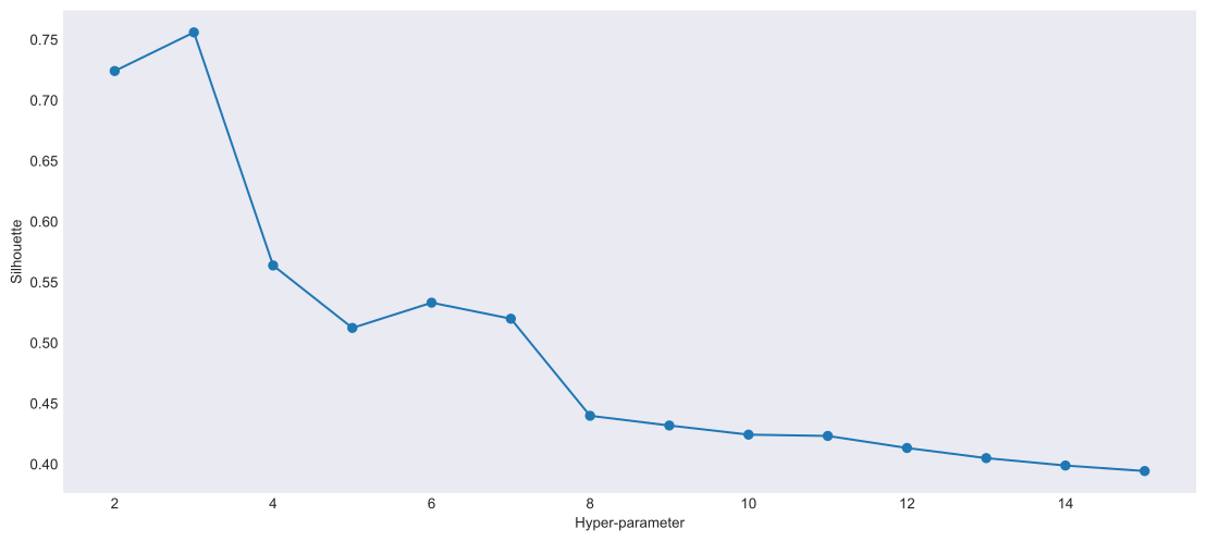
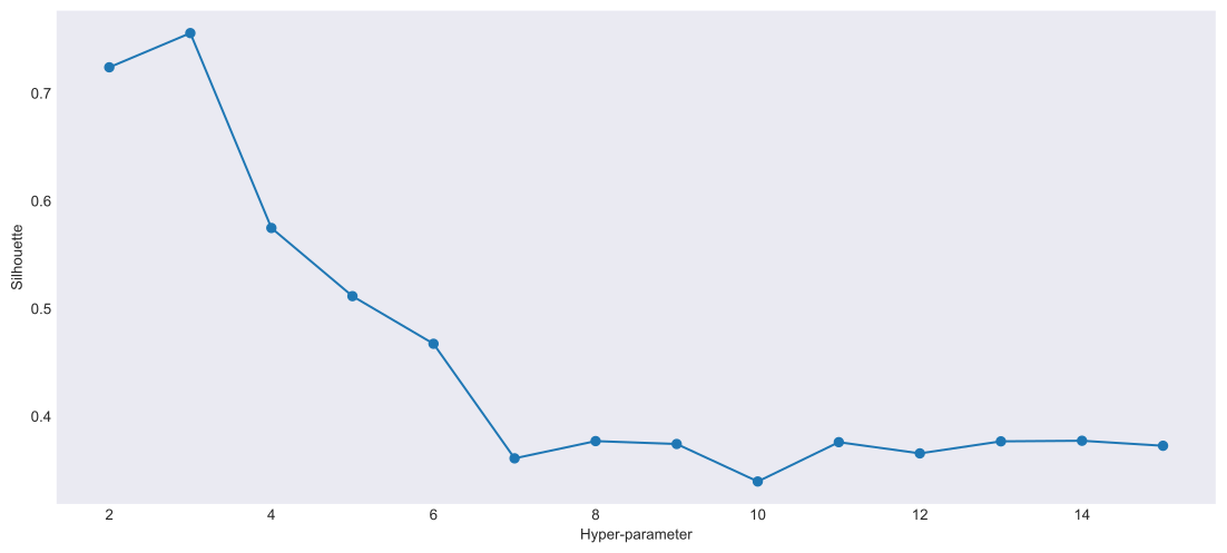
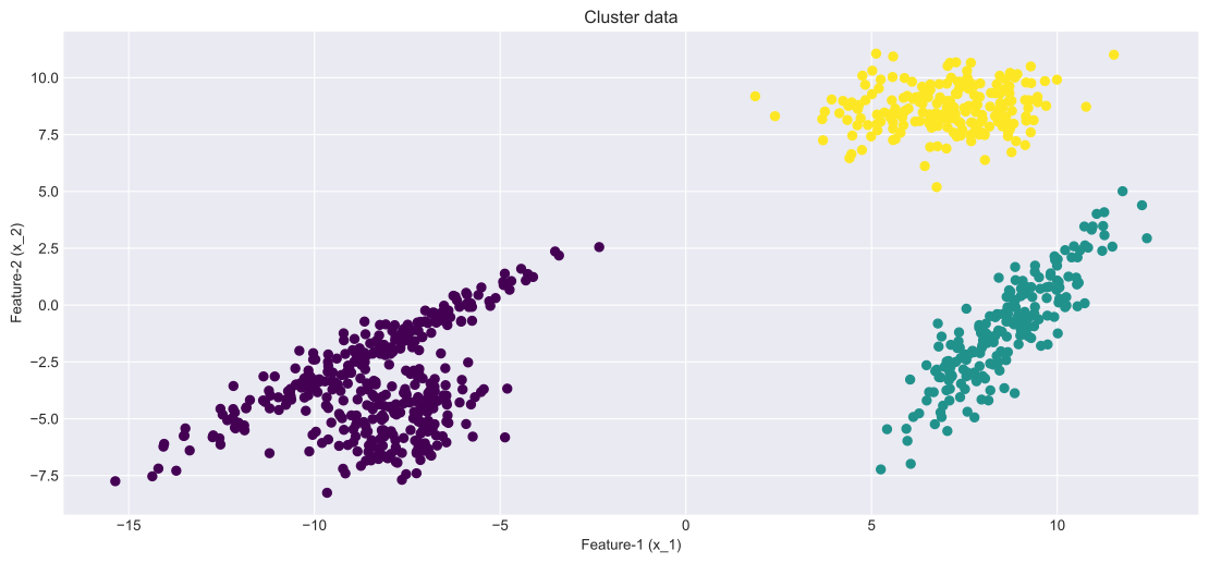
opt_labels=maximize_silhouette(X,algo="kmeans",nmax=15, i_plot=True)
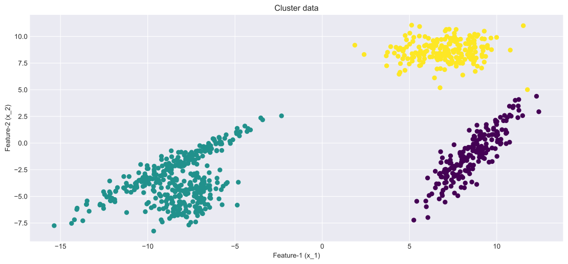
plot(X,opt_labels)
OPTIMAL PARAMETER = 3

AGGLOMERATIVE CLUSTERING

Code
# AGGLOMERATIVE CLUSTERING
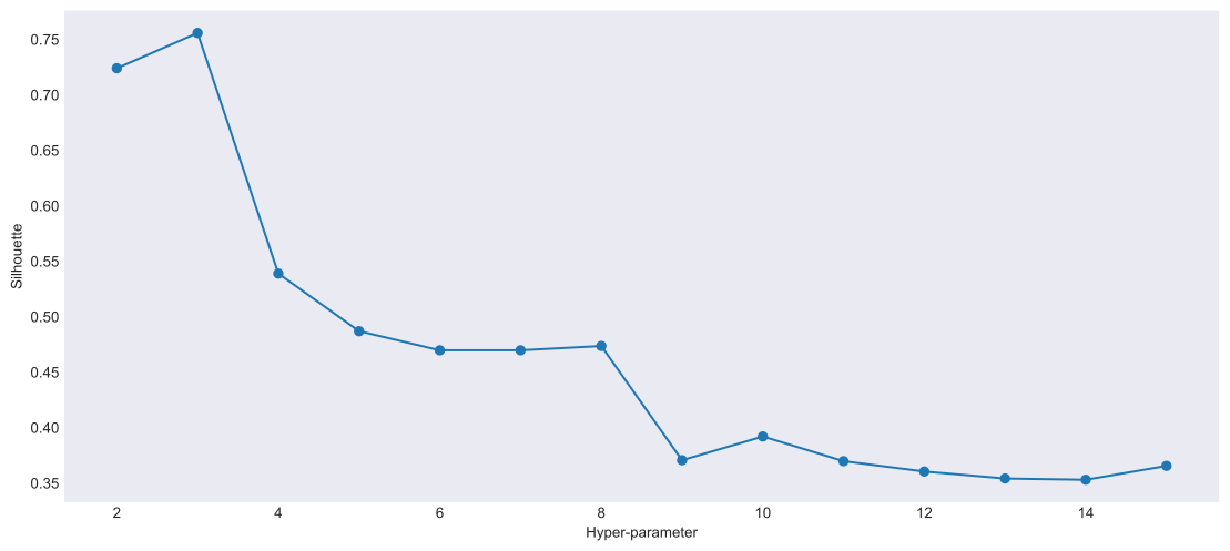
opt_labels=maximize_silhouette(X,algo="ag",nmax=15, i_plot=True)
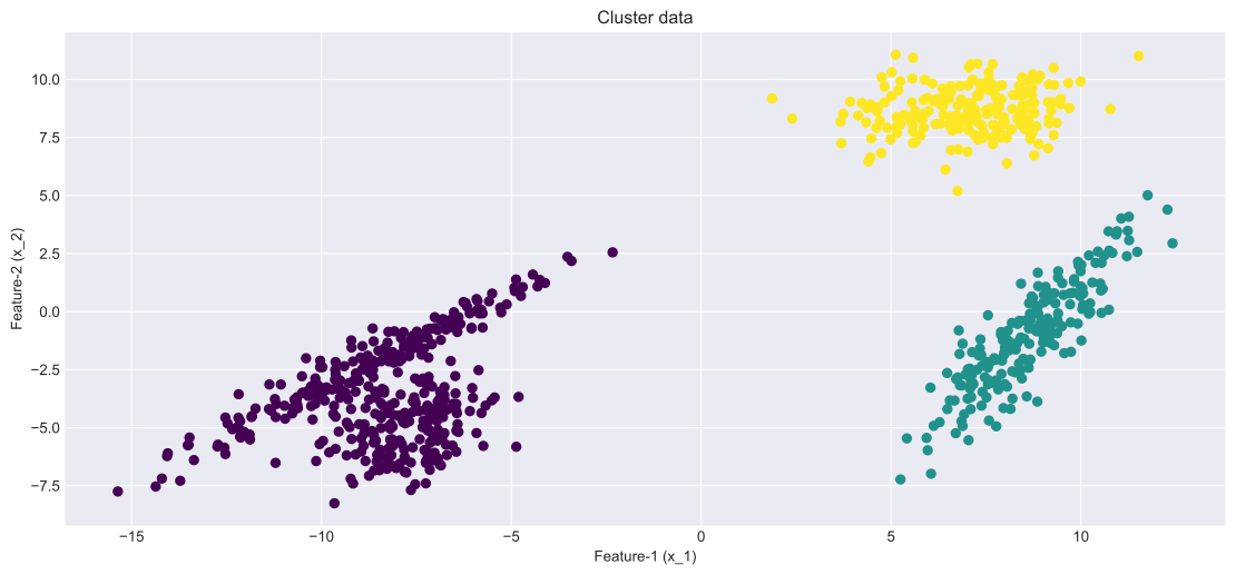
plot(X,opt_labels)
OPTIMAL PARAMETER = 3

DBSCAN

Code
# DBSCAN
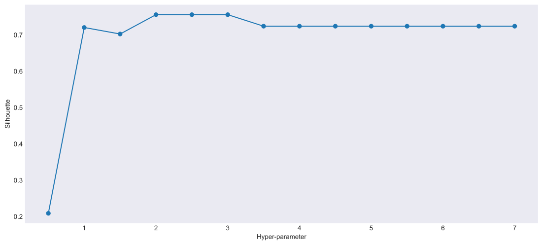
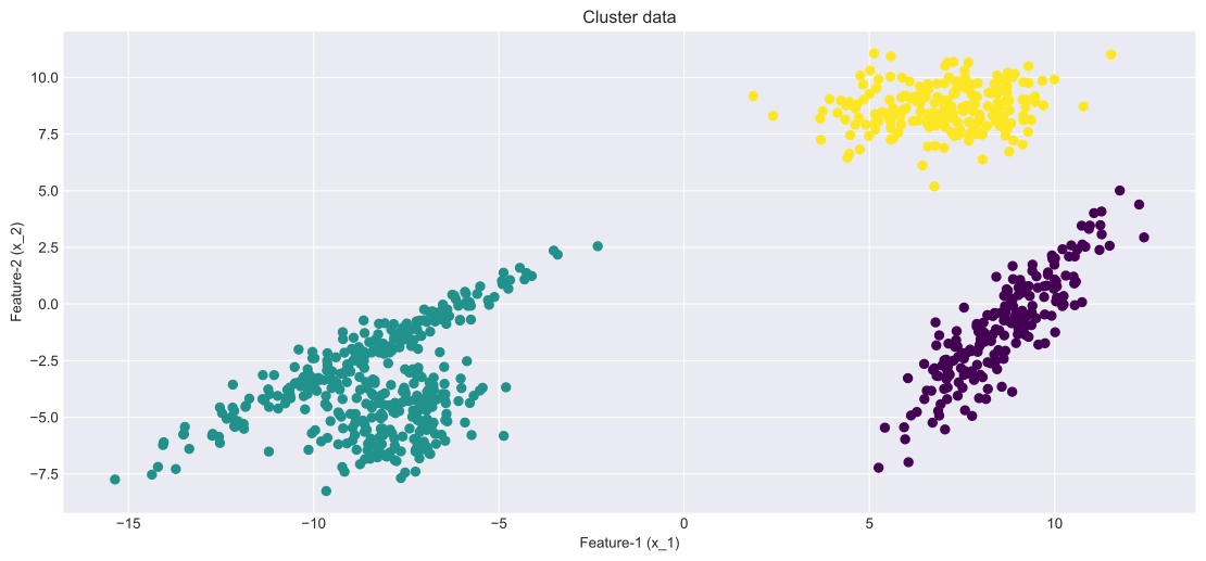
opt_labels=maximize_silhouette(X,algo="dbscan",nmax=15, i_plot=True)
plot(X,opt_labels)
OPTIMAL PARAMETER = 2.0

BIRCH

Code
# BIRCH
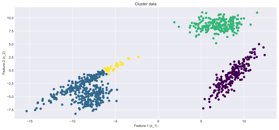
opt_labels=maximize_silhouette(X,algo="birch",nmax=15, i_plot=True)
plot(X,opt_labels)
OPTIMAL PARAMETER = 3

Run with “true” number of clusters

Obviously we typically won’t know the “true” number of labels in real-world situations

Code
# KMEANS
model = sklearn.cluster.KMeans(n_clusters=num_clusters_real).fit(X)
labels=model.predict(X)
plot(X,labels)

Code
# Birch
model = sklearn.cluster.Birch(n_clusters=num_clusters_real).fit(X)
labels=model.predict(X)
plot(X,labels)

Code
# KMEANS
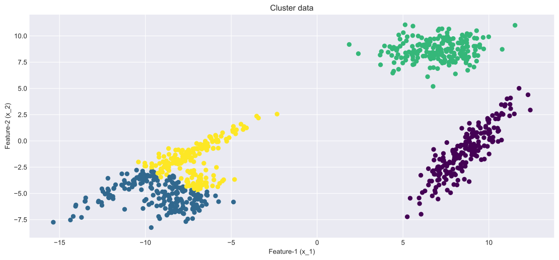
model = sklearn.cluster.AgglomerativeClustering(n_clusters=num_clusters_real).fit(X)
labels=model.labels_
plot(X,labels)

Code example:

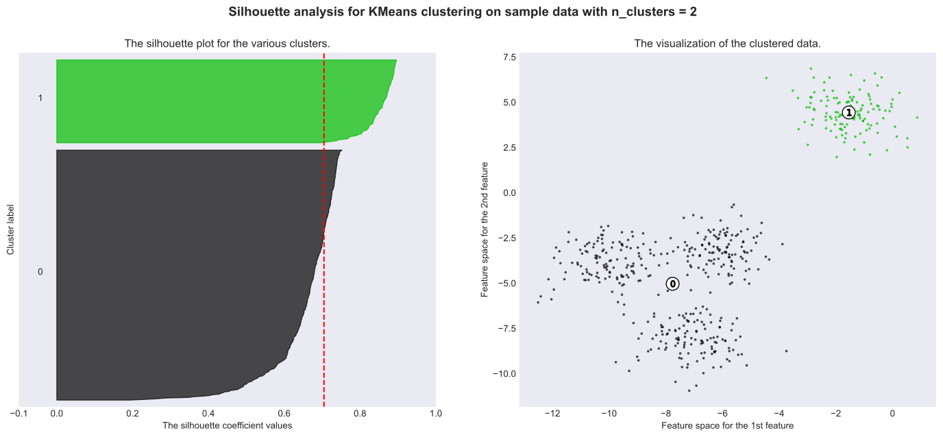
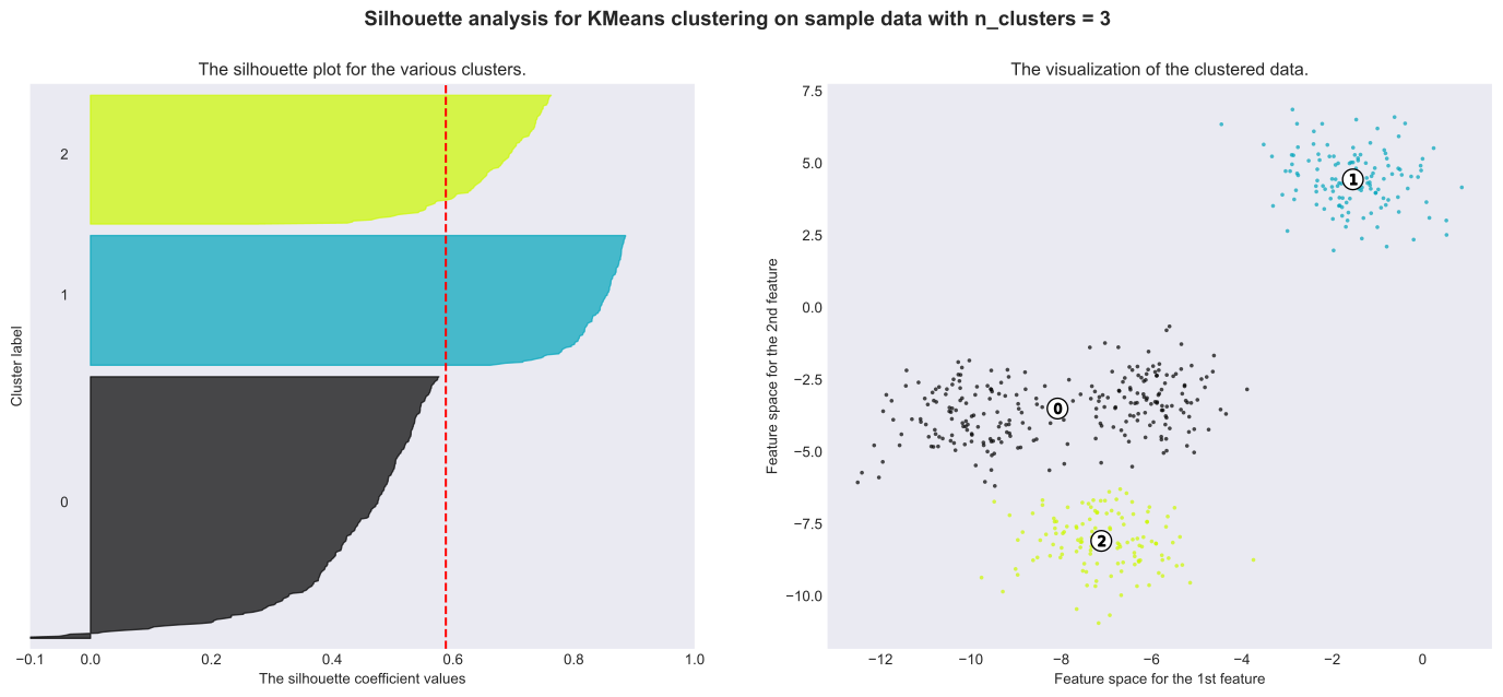
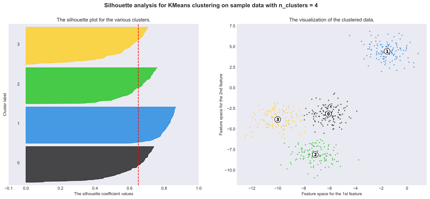
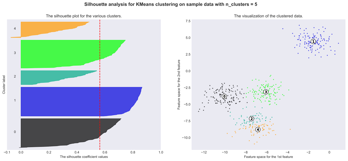
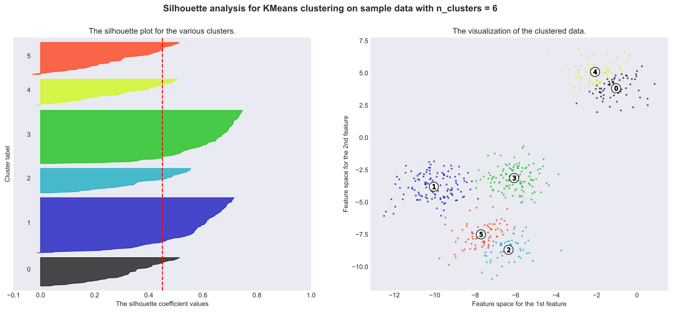
  • Bad choices: 3, 5 and 6 are a bad pick (below average silhouette scores)
  • Better choices: Silhouette analysis is more ambivalent in deciding between 2 and 4, however, 4 appears to be better.
Code
# SOURCE: https://scikit-learn.org/stable/auto_examples/cluster/plot_kmeans_silhouette_analysis.html

from sklearn.datasets import make_blobs
from sklearn.cluster import KMeans
from sklearn.metrics import silhouette_samples, silhouette_score

import matplotlib.pyplot as plt
import matplotlib.cm as cm
import numpy as np

# Generating the sample data from make_blobs
# This particular setting has one distinct cluster and 3 clusters placed close
# together.
X, y = make_blobs(
    n_samples=500,
    n_features=2,
    centers=4,
    cluster_std=1,
    center_box=(-10.0, 10.0),
    shuffle=True,
    random_state=1,
)  # For reproducibility

range_n_clusters = [2, 3, 4, 5, 6]

for n_clusters in range_n_clusters:
    # Create a subplot with 1 row and 2 columns
    fig, (ax1, ax2) = plt.subplots(1, 2)
    fig.set_size_inches(18, 7)

    # The 1st subplot is the silhouette plot
    # The silhouette coefficient can range from -1, 1 but in this example all
    # lie within [-0.1, 1]
    ax1.set_xlim([-0.1, 1])
    # The (n_clusters+1)*10 is for inserting blank space between silhouette
    # plots of individual clusters, to demarcate them clearly.
    ax1.set_ylim([0, len(X) + (n_clusters + 1) * 10])

    # Initialize the clusterer with n_clusters value and a random generator
    # seed of 10 for reproducibility.
    clusterer = KMeans(n_clusters=n_clusters, random_state=10)
    cluster_labels = clusterer.fit_predict(X)

    # The silhouette_score gives the average value for all the samples.
    # This gives a perspective into the density and separation of the formed
    # clusters
    silhouette_avg = silhouette_score(X, cluster_labels)
    print(
        "For n_clusters =",
        n_clusters,
        "The average silhouette_score is :",
        silhouette_avg,
    )

    # Compute the silhouette scores for each sample
    sample_silhouette_values = silhouette_samples(X, cluster_labels)

    y_lower = 10
    for i in range(n_clusters):
        # Aggregate the silhouette scores for samples belonging to
        # cluster i, and sort them
        ith_cluster_silhouette_values = sample_silhouette_values[cluster_labels == i]

        ith_cluster_silhouette_values.sort()

        size_cluster_i = ith_cluster_silhouette_values.shape[0]
        y_upper = y_lower + size_cluster_i

        color = cm.nipy_spectral(float(i) / n_clusters)
        ax1.fill_betweenx(
            np.arange(y_lower, y_upper),
            0,
            ith_cluster_silhouette_values,
            facecolor=color,
            edgecolor=color,
            alpha=0.7,
        )

        # Label the silhouette plots with their cluster numbers at the middle
        ax1.text(-0.05, y_lower + 0.5 * size_cluster_i, str(i))

        # Compute the new y_lower for next plot
        y_lower = y_upper + 10  # 10 for the 0 samples

    ax1.set_title("The silhouette plot for the various clusters.")
    ax1.set_xlabel("The silhouette coefficient values")
    ax1.set_ylabel("Cluster label")

    # The vertical line for average silhouette score of all the values
    ax1.axvline(x=silhouette_avg, color="red", linestyle="--")

    ax1.set_yticks([])  # Clear the yaxis labels / ticks
    ax1.set_xticks([-0.1, 0, 0.2, 0.4, 0.6, 0.8, 1])

    # 2nd Plot showing the actual clusters formed
    colors = cm.nipy_spectral(cluster_labels.astype(float) / n_clusters)
    ax2.scatter(
        X[:, 0], X[:, 1], marker=".", s=30, lw=0, alpha=0.7, c=colors, edgecolor="k"
    )

    # Labeling the clusters
    centers = clusterer.cluster_centers_
    # Draw white circles at cluster centers
    ax2.scatter(
        centers[:, 0],
        centers[:, 1],
        marker="o",
        c="white",
        alpha=1,
        s=200,
        edgecolor="k",
    )

    for i, c in enumerate(centers):
        ax2.scatter(c[0], c[1], marker="$%d$" % i, alpha=1, s=50, edgecolor="k")

    ax2.set_title("The visualization of the clustered data.")
    ax2.set_xlabel("Feature space for the 1st feature")
    ax2.set_ylabel("Feature space for the 2nd feature")

    plt.suptitle(
        "Silhouette analysis for KMeans clustering on sample data with n_clusters = %d"
        % n_clusters,
        fontsize=14,
        fontweight="bold",
    )

plt.show()
For n_clusters = 2 The average silhouette_score is : 0.7049787496083262
For n_clusters = 3 The average silhouette_score is : 0.5882004012129721
For n_clusters = 4 The average silhouette_score is : 0.6505186632729437
For n_clusters = 5 The average silhouette_score is : 0.56376469026194
For n_clusters = 6 The average silhouette_score is : 0.4504666294372765
Algorithm comparison code:

SOURCE: https://scikit-learn.org/stable/auto_examples/cluster/plot_cluster_comparison.html

Code
# SOURCE: https://scikit-learn.org/stable/auto_examples/cluster/plot_cluster_comparison.html

import time
import warnings

import numpy as np
import matplotlib.pyplot as plt

from sklearn import cluster, datasets, mixture
from sklearn.neighbors import kneighbors_graph
from sklearn.preprocessing import StandardScaler
from itertools import cycle, islice

np.random.seed(0)

# ============
# Generate datasets. We choose the size big enough to see the scalability
# of the algorithms, but not too big to avoid too long running times
# ============
n_samples = 500
noisy_circles = datasets.make_circles(n_samples=n_samples, factor=0.5, noise=0.05)
noisy_moons = datasets.make_moons(n_samples=n_samples, noise=0.05)
blobs = datasets.make_blobs(n_samples=n_samples, random_state=8)
no_structure = np.random.rand(n_samples, 2), None

# Anisotropicly distributed data
random_state = 170
X, y = datasets.make_blobs(n_samples=n_samples, random_state=random_state)
transformation = [[0.6, -0.6], [-0.4, 0.8]]
X_aniso = np.dot(X, transformation)
aniso = (X_aniso, y)

# blobs with varied variances
varied = datasets.make_blobs(
    n_samples=n_samples, cluster_std=[1.0, 2.5, 0.5], random_state=random_state
)

# ============
# Set up cluster parameters
# ============
plt.figure(figsize=(9 * 2 + 3, 13))
plt.subplots_adjust(
    left=0.02, right=0.98, bottom=0.001, top=0.95, wspace=0.05, hspace=0.01
)

plot_num = 1

default_base = {
    "quantile": 0.3,
    "eps": 0.3,
    "damping": 0.9,
    "preference": -200,
    "n_neighbors": 3,
    "n_clusters": 3,
    "min_samples": 7,
    "xi": 0.05,
    "min_cluster_size": 0.1,
}

datasets = [
    (
        noisy_circles,
        {
            "damping": 0.77,
            "preference": -240,
            "quantile": 0.2,
            "n_clusters": 2,
            "min_samples": 7,
            "xi": 0.08,
        },
    ),
    (
        noisy_moons,
        {
            "damping": 0.75,
            "preference": -220,
            "n_clusters": 2,
            "min_samples": 7,
            "xi": 0.1,
        },
    ),
    (
        varied,
        {
            "eps": 0.18,
            "n_neighbors": 2,
            "min_samples": 7,
            "xi": 0.01,
            "min_cluster_size": 0.2,
        },
    ),
    (
        aniso,
        {
            "eps": 0.15,
            "n_neighbors": 2,
            "min_samples": 7,
            "xi": 0.1,
            "min_cluster_size": 0.2,
        },
    ),
    (blobs, {"min_samples": 7, "xi": 0.1, "min_cluster_size": 0.2}),
    (no_structure, {}),
]

for i_dataset, (dataset, algo_params) in enumerate(datasets):
    # update parameters with dataset-specific values
    params = default_base.copy()
    params.update(algo_params)

    X, y = dataset

    # normalize dataset for easier parameter selection
    X = StandardScaler().fit_transform(X)

    # estimate bandwidth for mean shift
    bandwidth = cluster.estimate_bandwidth(X, quantile=params["quantile"])

    # connectivity matrix for structured Ward
    connectivity = kneighbors_graph(
        X, n_neighbors=params["n_neighbors"], include_self=False
    )
    # make connectivity symmetric
    connectivity = 0.5 * (connectivity + connectivity.T)
    # ============
    # Create cluster objects
    # ============
    ms = cluster.MeanShift(bandwidth=bandwidth, bin_seeding=True)
    two_means = cluster.MiniBatchKMeans(n_clusters=params["n_clusters"])
    ward = cluster.AgglomerativeClustering(
        n_clusters=params["n_clusters"], linkage="ward", connectivity=connectivity
    )
    spectral = cluster.SpectralClustering(
        n_clusters=params["n_clusters"],
        eigen_solver="arpack",
        affinity="nearest_neighbors",
    )
    dbscan = cluster.DBSCAN(eps=params["eps"])
    optics = cluster.OPTICS(
        min_samples=params["min_samples"],
        xi=params["xi"],
        min_cluster_size=params["min_cluster_size"],
    )
    affinity_propagation = cluster.AffinityPropagation(
        damping=params["damping"], preference=params["preference"], random_state=0
    )
    average_linkage = cluster.AgglomerativeClustering(
        linkage="average",
        affinity="cityblock",
        n_clusters=params["n_clusters"],
        connectivity=connectivity,
    )
    birch = cluster.Birch(n_clusters=params["n_clusters"])
    gmm = mixture.GaussianMixture(
        n_components=params["n_clusters"], covariance_type="full"
    )

    clustering_algorithms = (
        ("MiniBatch\nKMeans", two_means),
        ("Affinity\nPropagation", affinity_propagation),
        ("MeanShift", ms),
        ("Spectral\nClustering", spectral),
        ("Ward", ward),
        ("Agglomerative\nClustering", average_linkage),
        ("DBSCAN", dbscan),
        ("OPTICS", optics),
        ("BIRCH", birch),
        ("Gaussian\nMixture", gmm),
    )

    for name, algorithm in clustering_algorithms:
        t0 = time.time()

        # catch warnings related to kneighbors_graph
        with warnings.catch_warnings():
            warnings.filterwarnings(
                "ignore",
                message="the number of connected components of the "
                + "connectivity matrix is [0-9]{1,2}"
                + " > 1. Completing it to avoid stopping the tree early.",
                category=UserWarning,
            )
            warnings.filterwarnings(
                "ignore",
                message="Graph is not fully connected, spectral embedding"
                + " may not work as expected.",
                category=UserWarning,
            )
            algorithm.fit(X)

        t1 = time.time()
        if hasattr(algorithm, "labels_"):
            y_pred = algorithm.labels_.astype(int)
        else:
            y_pred = algorithm.predict(X)

        plt.subplot(len(datasets), len(clustering_algorithms), plot_num)
        if i_dataset == 0:
            plt.title(name, size=18)

        colors = np.array(
            list(
                islice(
                    cycle(
                        [
                            "#377eb8",
                            "#ff7f00",
                            "#4daf4a",
                            "#f781bf",
                            "#a65628",
                            "#984ea3",
                            "#999999",
                            "#e41a1c",
                            "#dede00",
                        ]
                    ),
                    int(max(y_pred) + 1),
                )
            )
        )
        # add black color for outliers (if any)
        colors = np.append(colors, ["#000000"])
        plt.scatter(X[:, 0], X[:, 1], s=10, color=colors[y_pred])

        plt.xlim(-2.5, 2.5)
        plt.ylim(-2.5, 2.5)
        plt.xticks(())
        plt.yticks(())
        plt.text(
            0.99,
            0.01,
            ("%.2fs" % (t1 - t0)).lstrip("0"),
            transform=plt.gca().transAxes,
            size=15,
            horizontalalignment="right",
        )
        plot_num += 1

plt.show()