Networks of physical particles
Simulating the dynamic evolution of systems of interacting particles 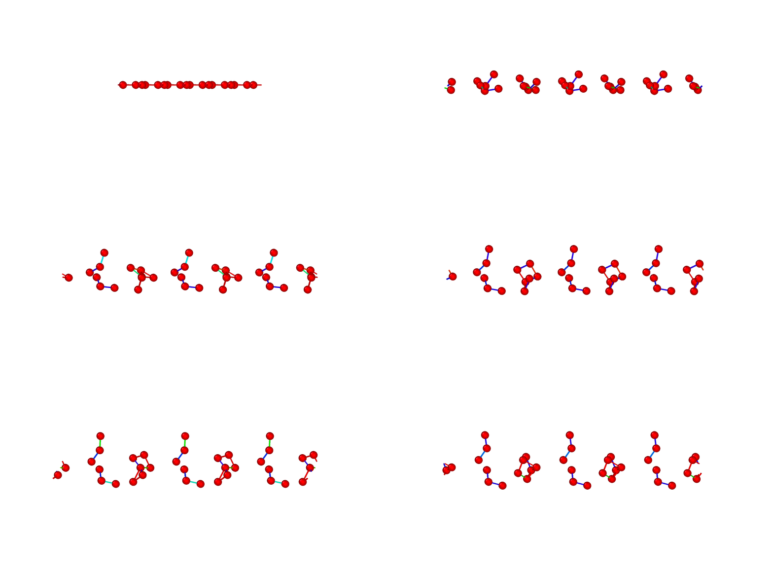
Particle system example-1
The same governing physical laws (Newton’s laws \(\mathbf F_i=m_i \mathbf a_i\)), can be applied to a wide range of phenomena
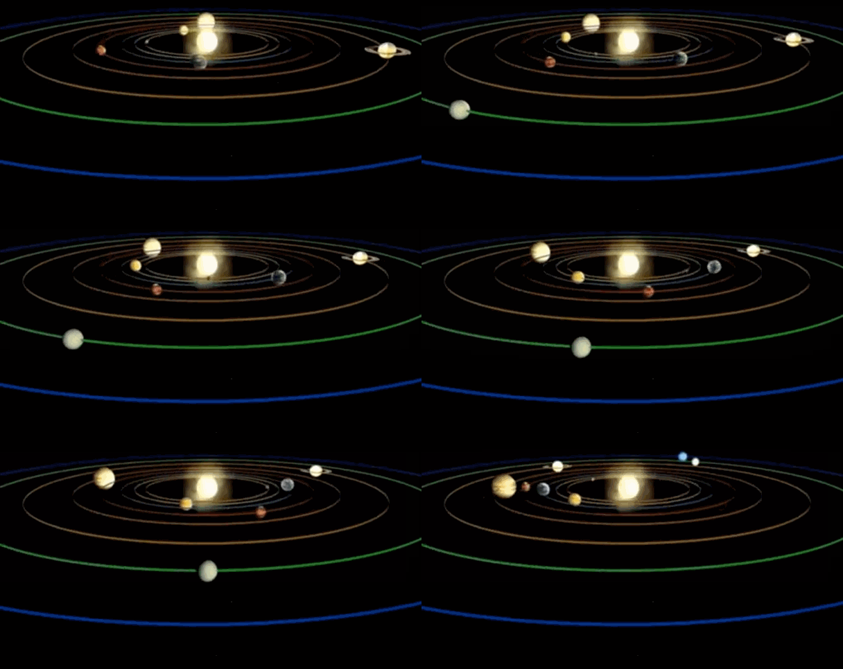
Orbital systems
- Planets, rockets, and asteroids are collections of particles, governed by \(\mathbf F_i=m_i \mathbf a_i\), interacting via gravitational forces.
Atomic and molecular systems
- From a classical perspective, At the atomic level the particles follow the same rules, however, in this case, the forces are inter-atomic chemical bonds rather than gravitational forces

Explore publications!!!
Particle system example-2
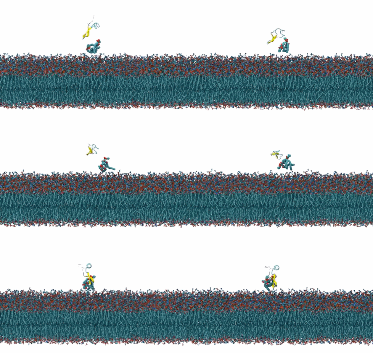
Bio-physics: We use the same methods for biological molecules (e.g. protein folding, drug delivery, lipid bi-layers, etc)
Newtonian worldview:
- The following are the
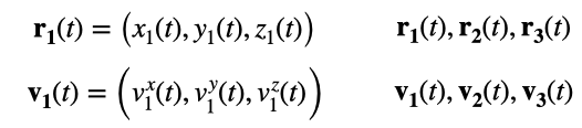
fundamental quantitiesin the Newtonian worldview.
- This shows static
snapshotof the system in time.
![]()
- In this case the
nodes=particlesandedges=bonds, generally these quantities will have a temporal dependence.2D:\(\mathbf{r}_i(t)=(x_i(t),y_i(t))\) or3D:\(\mathbf{r}_i(t)=(x_i(t),y_i(t),z_i(t))\)
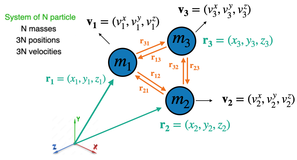
Additional quantities
kinetic energy: \(k_i=\frac{1}{2} m\left|\mathbf{v}_{\mathbf{i}}\right|^2=\frac{1}{2} m\left(v_x^2+v_y^2+v_z^2\right) \quad \mathrm{N}\) kinetic energiespotential energy: \(u_i=u\left(\mathbf{r}_i\right)\) potential energy (describes particle-interactions)- Total configurational potential energy \(=U\left(\mathbf{r}_1, \mathbf{r}_2, \mathbf{r}_3\right)\)
- Total energy \(E_{t o t}=\sum_{i=1}^N m_i \frac{\mathbf{v}_i^2}{2}+U\left(\mathbf{r}_1, \ldots, \mathbf{r}_N\right)\)
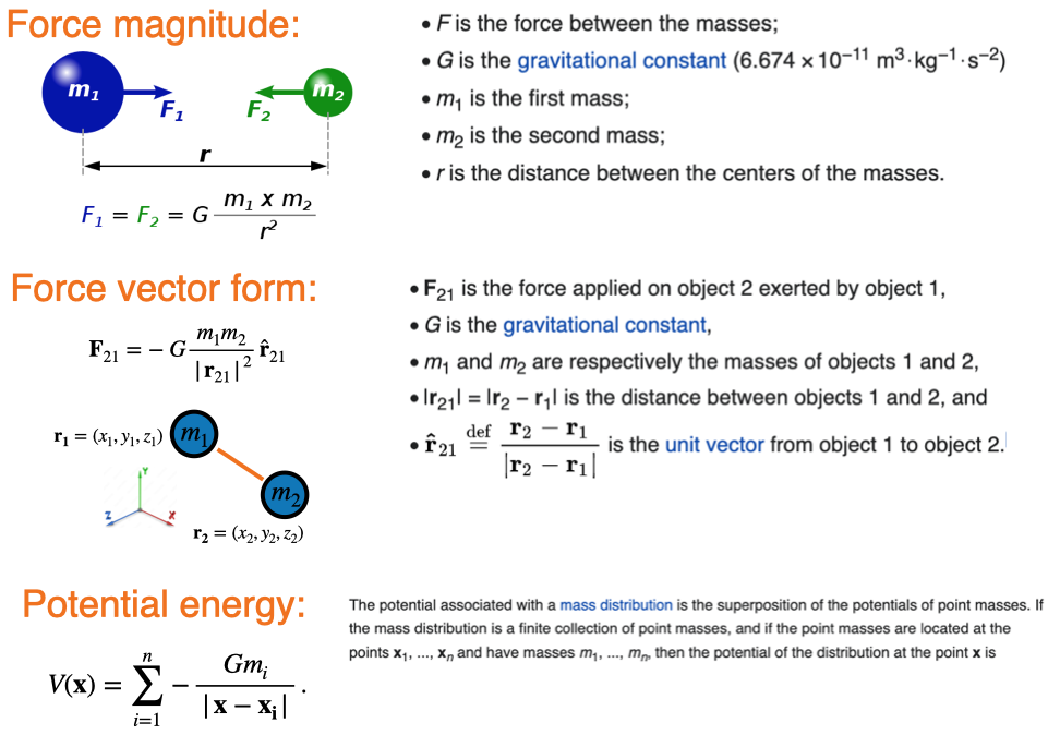
Gravitational Forces
- Forces make things move, i.e. cause an acceleration \(\mathbf F_i=m_i \mathbf a_i\)
- For gravitational interactions, the forces can be calculated directly from the relative positions of the nodes (particles)
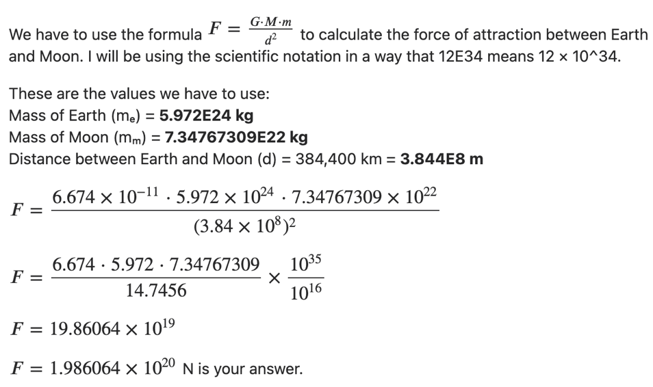
Example:
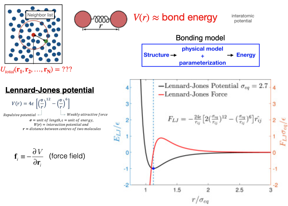
Interatomic Forces
- For simple elements, e.g. noble gases, the bonding energy can be accurately approximated via physically derived parametric models
Newtonian worldview: Dynamic evolution
- If you can compute the forces on every particle in the simulation at a particular point in time, then you can extract the associated accelerations at that time.
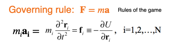
- The acceleration can be used to progress the system forward in time to
predict futurepositions and velocities
Molecular Dynamics
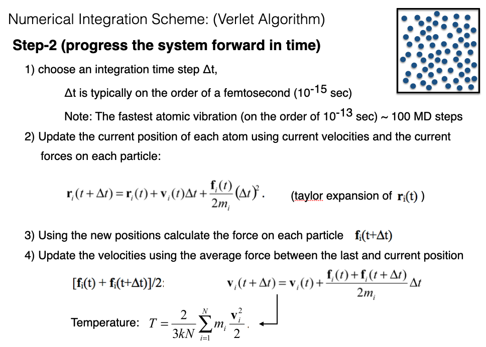
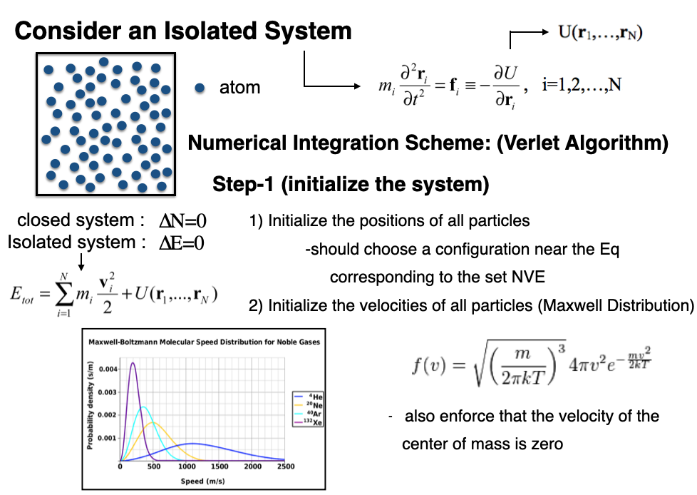
- The algorithm to progress the system forward in time is known as
Molecular Dynamics - One common methods to update the positions, and velocities is called the
Velocity-Verletalgorithm![]()
Molecular Dynamics: Continued