In mathematics, a system of linear equations (or linear system) is a collection of one or more linear equations involving the same variables. \({ }^{[1]}\)
is a system of three equations in the three variables \(x, y, z\). A solution to a linear system is an assignment of values to the variables such that all the equations are simultaneously satisfied. In the example above, a solution is given by the ordered triple \((x, y, z)=(1,-2,-2)\), since it makes all three equations valid.
The word “system” indicates that the equations should be considered collectively, rather than individually.
Source: Wikipedia
Analytical methods
Analytical methods for solving linear equations involve algebraic manipulation to find the exact solution. These methods typically include:
Direct Methods: Such as Gaussian elimination, LU decomposition, and Cholesky decomposition. These methods find the exact solution by performing a series of mathematical operations on the equations.
Matrix Inversion: Involves finding the inverse of the coefficient matrix and then multiplying it by the constant vector. This method is computationally expensive for large matrices.
Cramer’s Rule: Provides a formulaic method for solving systems of linear equations using determinants.
Analytical methods guarantee the exact solution to the linear equations but may become impractical for large systems due to computational complexity.
Connecting with linear algebra and Matrix Inversion
The same three equations, stacked, are a single matrix equation \(A\mathbf{x} = \mathbf{b}\): coefficients go in \(A\), unknowns in \(\mathbf{x}\), right-hand sides in \(\mathbf{b}\).
Row \(i\) of \(A\) holds the coefficients of equation \(i\); multiplying it across \(\mathbf{x}\) rebuilds that equation’s left side. So \(A\mathbf{x} = \mathbf{b}\) is just all three equations enforced at once.
Solve by inversion. If \(A\) is invertible, left-multiply both sides by \(A^{-1}\):
For this system the unique solution is \((x, y, z) = (1, -2, -2)\), which satisfies all three equations simultaneously.
When it works. Inversion gives a single solution only when \(A\) is nonsingular (\(\det A \neq 0\)). A singular \(A\) means no unique solution, and the inverse does not exist.
Iterative Methods
Methods for iteratively solving linear equations include:
Jacobi Iteration: Updates each variable using the previous iteration’s values for all other variables.
Gauss-Seidel Iteration: Similar to Jacobi, but uses updated values for variables as soon as they are available.
Successive Over-Relaxation (SOR): A modification of Gauss-Seidel with a relaxation parameter to accelerate convergence.
Conjugate Gradient Method: Iteratively minimizes a quadratic function, often used for symmetric positive definite matrices.
Iterative Refinement: Applies a direct method iteratively to improve the solution’s accuracy.
Krylov Subspace Methods: Iteratively solve linear systems using subspaces spanned by the initial residual and matrix powers.
Source: GPT3.5
Jacobi Method: Solve Each Equation for Its Own Variable
Goal: solve \(A\mathbf{x} = \mathbf{b}\) without ever inverting \(A\), by guessing and refining.
The trick: equation \(i\) is the only one with \(x_i\) on its diagonal, so solve that row for \(x_i\) assuming every other variable is already known.
In words: take the right-hand side \(b_i\), subtract off what all the other variables contribute, and divide by your own diagonal coefficient. That gives an updated guess for \(x_i\).
Start from any guess (often all zeros), apply this to every row at once, and repeat. Each sweep nudges the whole vector closer to the true solution.
Why it converges: if each variable dominates its own equation (the diagonal is large compared to the rest of its row), every update is mostly self-correcting, and the errors shrink each pass.
Jacobi: matrix form
Every variable updates using only the previous sweep’s values. The new vector \(\mathbf{x}^{(k+1)}\) is built entirely from the old \(\mathbf{x}^{(k)}\), never from values computed earlier in the same sweep.
Reading the matrix form: \(D\) is just the diagonal (the cheap, trivially invertible part), and \(L + U\) is everything off the diagonal (the coupling between variables). So \(D^{-1}\) undoes the easy part and \((L+U)\mathbf{x}^{(k)}\) carries in the cross-talk.
This freeze-the-old-values rule is the whole personality of Jacobi: because nothing depends on the order you process rows, every update is independent, so all \(n\) can be computed in parallel.
The cost is memory: you must keep both the old and the new vector, since the old one is still being read while the new one fills in. Minimum storage is two length-\(n\) vectors.
Gauss-Seidel is the one-line variant that drops this rule, overwriting each value the instant it is computed so later updates in the same sweep use fresher numbers. It needs only one vector and usually converges faster, at the price of being sequential.
Then \(A\) can be decomposed into a diagonal component \(D\), a lower triangular part \(L\) and an upper triangular part \(U\) : \[
A=D+L+U \quad \text { where } \quad D=\left[\begin{array}{cccc}
a_{11} & 0 & \cdots & 0 \\
0 & a_{22} & \cdots & 0 \\
\vdots & \vdots & \ddots & \vdots \\
0 & 0 & \cdots & a_{n n}
\end{array}\right] \text { and } L+U=\left[\begin{array}{cccc}
0 & a_{12} & \cdots & a_{1 n} \\
a_{21} & 0 & \cdots & a_{2 n} \\
\vdots & \vdots & \ddots & \vdots \\
a_{n 1} & a_{n 2} & \cdots & 0
\end{array}\right] \text {. }
\]
Example
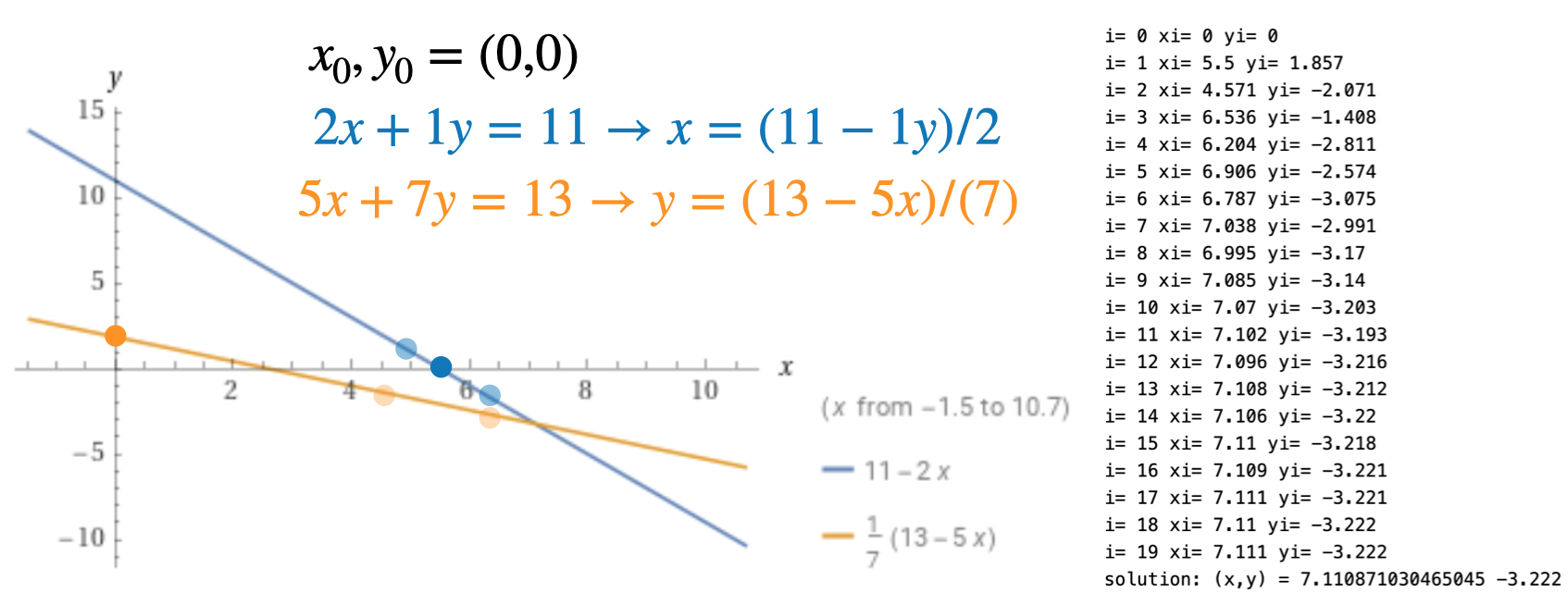
A linear system of the form \(A x=b\) with initial estimate \(x^{(0)}\) is given by \[
A=\left[\begin{array}{ll}
2 & 1 \\
5 & 7
\end{array}\right], b=\left[\begin{array}{l}
11 \\
13
\end{array}\right] \quad \text { and } \quad x^{(0)}=\left[\begin{array}{l}
1 \\
1
\end{array}\right] .
\]
import numpy as np# initial guessxi=0yi=0# iterative solutionfor i inrange(0,20):#print(np.round(np.array([xi,yi])))# Jacobi Iteration or Gauss-Seidel method="J"print("i=",i,"xi=",np.round(xi,3),"yi=",np.round(yi,3))if method=="J":# apply formula xip1=(11.-1*yi)/2.0 yip1=(13-5.*xi)/(7.0)# update xi=xip1 yi=yip1else:# apply formula (in place update) xi=(11.-1*yi)/2.0 yi=(13-5.*xi)/(7.0)print("solution: (x,y) =",xi,yi)
import numpy as np# initial guessxi=0.0yi=0.0# iterative solutionfor i inrange(0,5):print(np.round(np.array([xi,yi]),2))# Jacobi Iteration or Gauss-Seidel# xi=(2-yi)/3.# yi=(1-xi)/4. xip1=1-4*yi yip1=2.-3*xi xi=xip1 yi=yip1# [3 1] 2# [1 4] 1# 3x+1y=2# 1x+4y=1 # Gauss-Seidel is an iterative method used to solve linear systems of equations, particularly when the matrix involved is diagonally dominant # A matrix is diagonally dominant if the magnitude of each diagonal element is greater than or equal to the sum of the magnitudes of the other elements in the same row (or column),print("solution: (x,y) =",xi,yi)print("x,y",7/11.,1./11)
The minimum is exactly where the gradient vanishes, \(A\mathbf{x} = \mathbf{b}\), so minimizing \(f\) solves the system.
Why not just invert? For large sparse \(A\), forming \(A^{-1}\) costs about \(O(n^{3})\) and destroys sparsity. Conjugate gradient only ever needs matrix-vector products \(A\mathbf{p}\), which stay cheap when \(A\) is sparse.
The key trick. Plain steepest descent zig-zags down the bowl and undoes its own progress. CG instead picks search directions that are conjugate (A-orthogonal), so each step’s gain is never spoiled by the next.
Convergence. In exact arithmetic CG reaches the true solution in at most \(n\) steps, and usually gets close in far fewer, which is why it is the workhorse for huge symmetric systems.
Conjugate Gradient: Solver vs Optimizer
For a symmetric positive definite \(A\), solving \(A\mathbf{x} = \mathbf{b}\) and minimizing the quadratic \(f(\mathbf{x}) = \tfrac{1}{2}\mathbf{x}^{T}A\mathbf{x} - \mathbf{b}^{T}\mathbf{x}\) are the same problem: the minimum is exactly where \(\nabla f = A\mathbf{x} - \mathbf{b} = 0\). “Solver” and “optimizer” are two names for one algorithm.
Most common use: a linear solver. Large sparse SPD systems, above all the discretized PDEs of physics and engineering (heat, diffusion, structural mechanics), and graph Laplacian solves for resistance, embeddings, and diffusion.
Here CG (usually preconditioned) is the workhorse, and people rarely mention the quadratic at all.
The optimization framing dominates in ML. CG appears as the inner solve for a Newton step \(H\mathbf{p} = -\mathbf{g}\) in Hessian-free and trust-region methods, and its nonlinear cousins (Fletcher-Reeves, Polak-Ribiere) minimize general smooth objectives, not just quadratics.
Why it scales either way: CG only ever needs the action \(A\mathbf{p}\) (a matrix-vector product), never \(A^{-1}\) or even \(A\) itself. That matrix-free property is what lets it handle millions of unknowns and slot into Hessian-free training.
Bottom line: solving a linear system is the more common use overall, the quadratic view is the cleaner way to understand and to optimize, and the choice of name is about what you set out to do, not a difference in the method.
Conjugate Gradient: A Worked 2x2 Example
Solve \(A\mathbf{x} = \mathbf{b}\) with a symmetric positive definite \(A\), starting from \(\mathbf{x}_0 = \mathbf{0}\):
Step 1 (steepest descent). The residual is \(\mathbf{r}_0 = \mathbf{b} - A\mathbf{x}_0 = (1, 2)\), and the first direction is \(\mathbf{p}_0 = \mathbf{r}_0\).
Step 2 (conjugate correction). The new residual is \(\mathbf{r}_1 = (-0.5,\, 0.25)\). CG does not just follow it; it bends the direction to stay conjugate to \(\mathbf{p}_0\):
Two unknowns, two steps. Check: \(4(\tfrac{1}{11}) + \tfrac{7}{11} = 1\) and \(\tfrac{1}{11} + 3(\tfrac{7}{11}) = 2\). The conjugate directions guarantee an exact hit in at most \(n\) steps, here \(n = 2\).
Optional assignment:
Repeat the process but for the simple system
Suppose we are given the following linear system: \[
\begin{aligned}
10 x_1-x_2+2 x_3 & =6, \\
-x_1+11 x_2-x_3+3 x_4 & =25, \\
2 x_1-x_2+10 x_3-x_4 & =-11, \\
3 x_2-x_3+8 x_4 & =15 .
\end{aligned}
\]
The exact solution of the system is (1, 2, −1, 1).