
Network structure

Source

Overview

  • In this section we focus on how to quantify the structure of a network.
  • Structure property relationship: In network science, the structure of a network often relates to its properties.
  • We will focus on the following properties:
    • Assortativity
    • Connectedness
    • Paths
    • Trees
    • Small-world property

Visualization of network structure

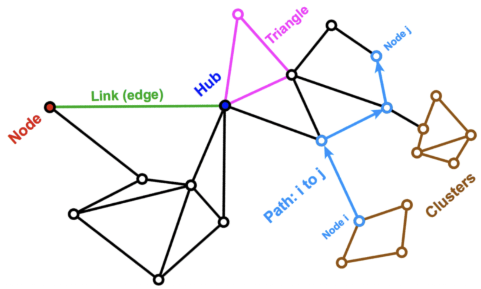
Here we show examples of common elements that emerge in network structures, we will be looking at each of these more closely as we go along.

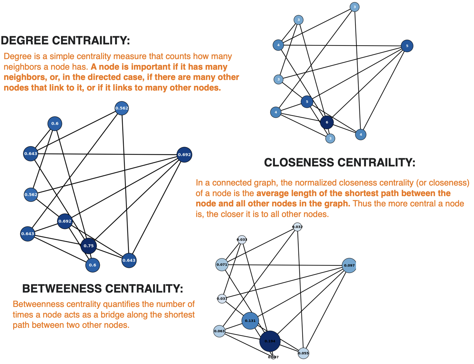
  • Recall centrality: Method to quantify the importance of a node or a link

Homophily and Assortativity

Birds of a feather flock together

Getting started: recall social networks

It is important to note that the following discussion primarily focuses on social networks.

While aspects of the discussion may be applied more generally, other types of networks, such as information networks, biological networks, and communication networks, may or maynot exhib similar properties.

Homophily: A network formation mechanism

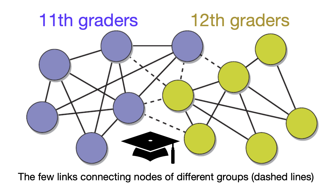
  • Definition: The tendency for similar individuals (nodes) to form connections more frequently than dissimilar ones.

*“Birds of a feather flock together.”

  • Examples: People with similar beliefs, professions, or cultural backgrounds often become friends.

  • Consequences:

    • Can strengthen communities and foster support.
    • But also contributes to echo chambers and filter bubbles, where exposure to diverse viewpoints is limited.
    • Increases a network’s vulnerability to misinformation and coordinated influence.

Social Influence

  • Definition: The process by which connected individuals become more similar over time due to interaction and mutual influence.

In some sense, social influence is the opposite of homophily, i.e. dissimilar nodes with existing connections becoming similar over time, rather than similar nodes forming connections (homophily).

  • Examples:

    • Friends adopting each other’s slang, habits, or political opinions.
    • Collective behavior shifts during trends or viral movements.

Chicken or the Egg?

  • Do we form links because we are similar (homophily), or do we become similar because we are linked (social influence)?

  • In most real-world networks, these forces:

    • Operate simultaneously,
    • Reinforce each other, and
    • Make it challenging to untangle cause from effect.

The dynamic interplay between homophily and influence shapes the structure and evolution of social networks.

Assortativity: Quantifying network similarity

  • Definition: Assortativity is a network property that measures the tendency of nodes in a network to connect to other nodes that are similar in some way.

  • Types of Assortativity:

    • Degree Assortativity: Do high-degree nodes connect to other high-degree nodes?
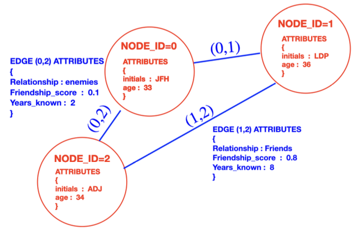
    • Attribute Assortativity: Do nodes with similar attributes (e.g., age, gender, profession) tend to connect?
  • Interpretation:

    • Positive Assortativity: Similar nodes are more likely to connect (e.g., friends with similar ages).
    • Negative Assortativity (Disassortativity): Dissimilar nodes are more likely to connect (e.g., mentors and mentees).
  • Importance:

    • Influences the robustness and dynamics of networks.
    • Helps understand patterns of segregation or integration.

Example: Attribute Assortativity

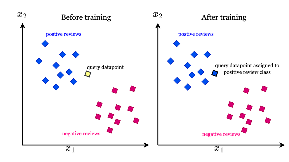
Assortativity increases predictive power:

  • If assortativity is present we can make predictions about attributes of unknown nodes by inspecting their neighbors

  • Conceptually this is a similar idea to the KNN algorithm in machine learning

Important: It is however still differnt, in KNN the “similarity” is entirely based on the features (attributes) of a data-point, since there are no edges, in network science we can use the network structure itself to make predictions.

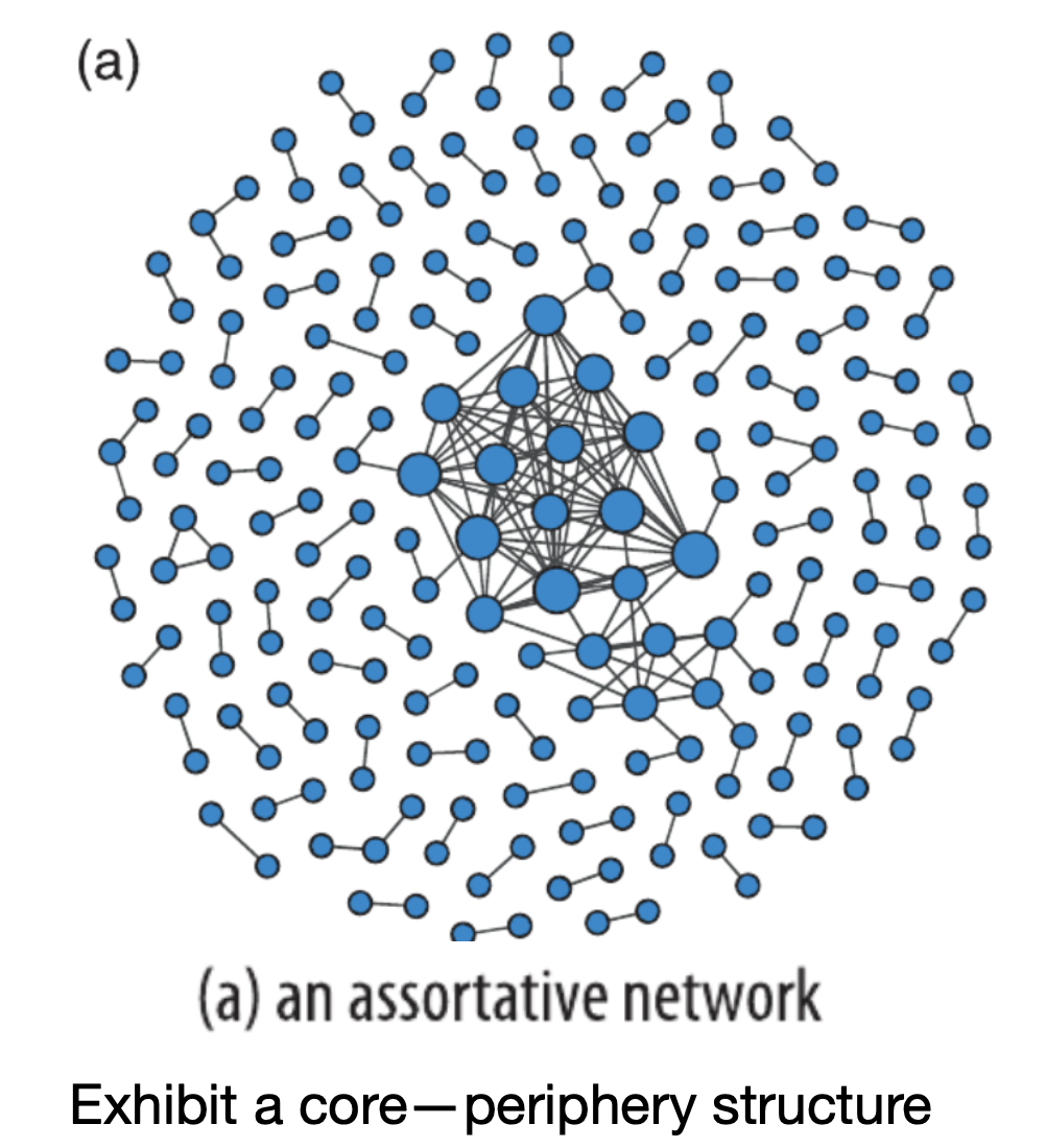
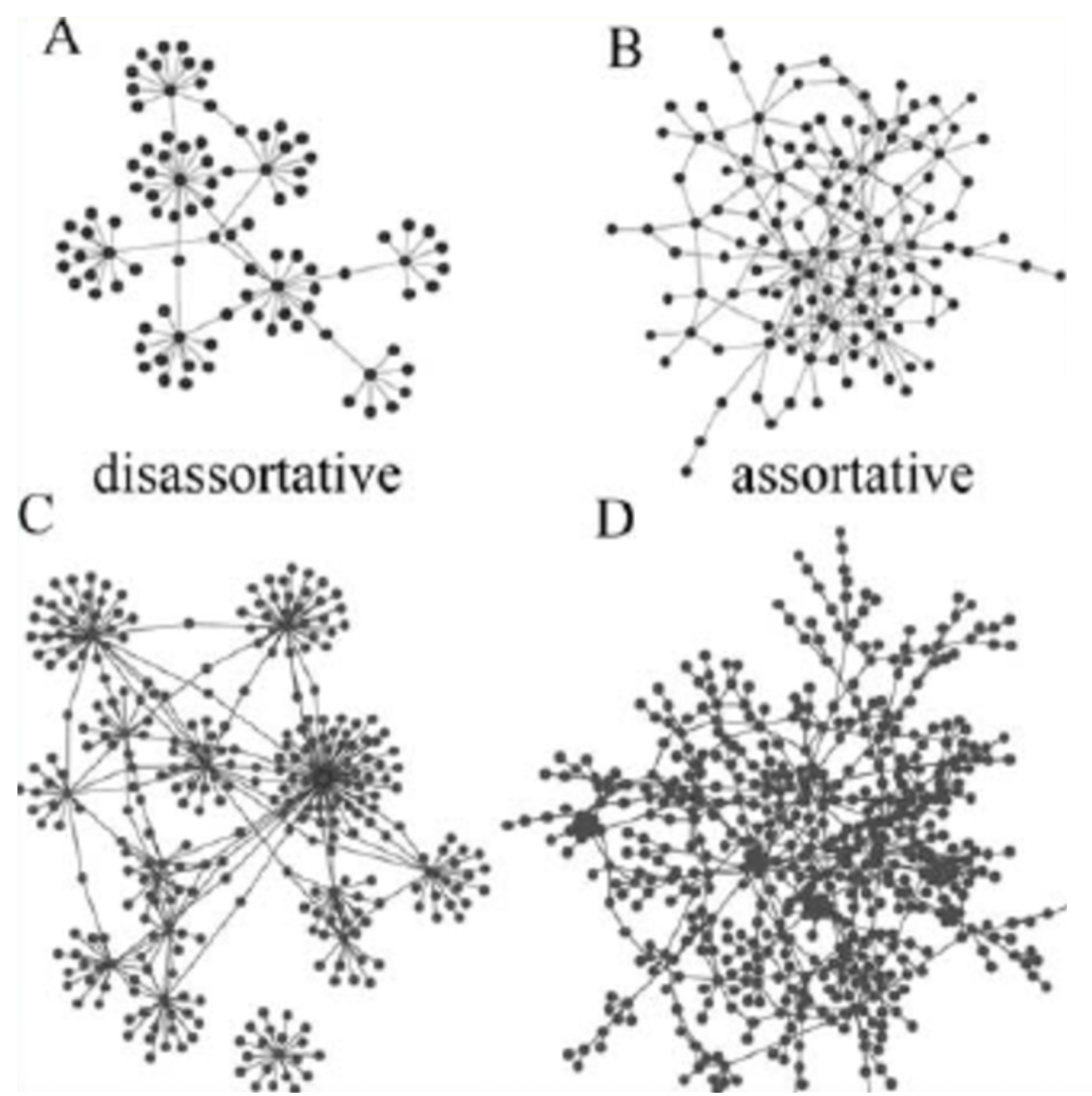
Example: Assortative networks

high-degree nodes tend to be connected to other high-degree nodes, while low-degree nodes tend to have other low-degree nodes as neighbors.

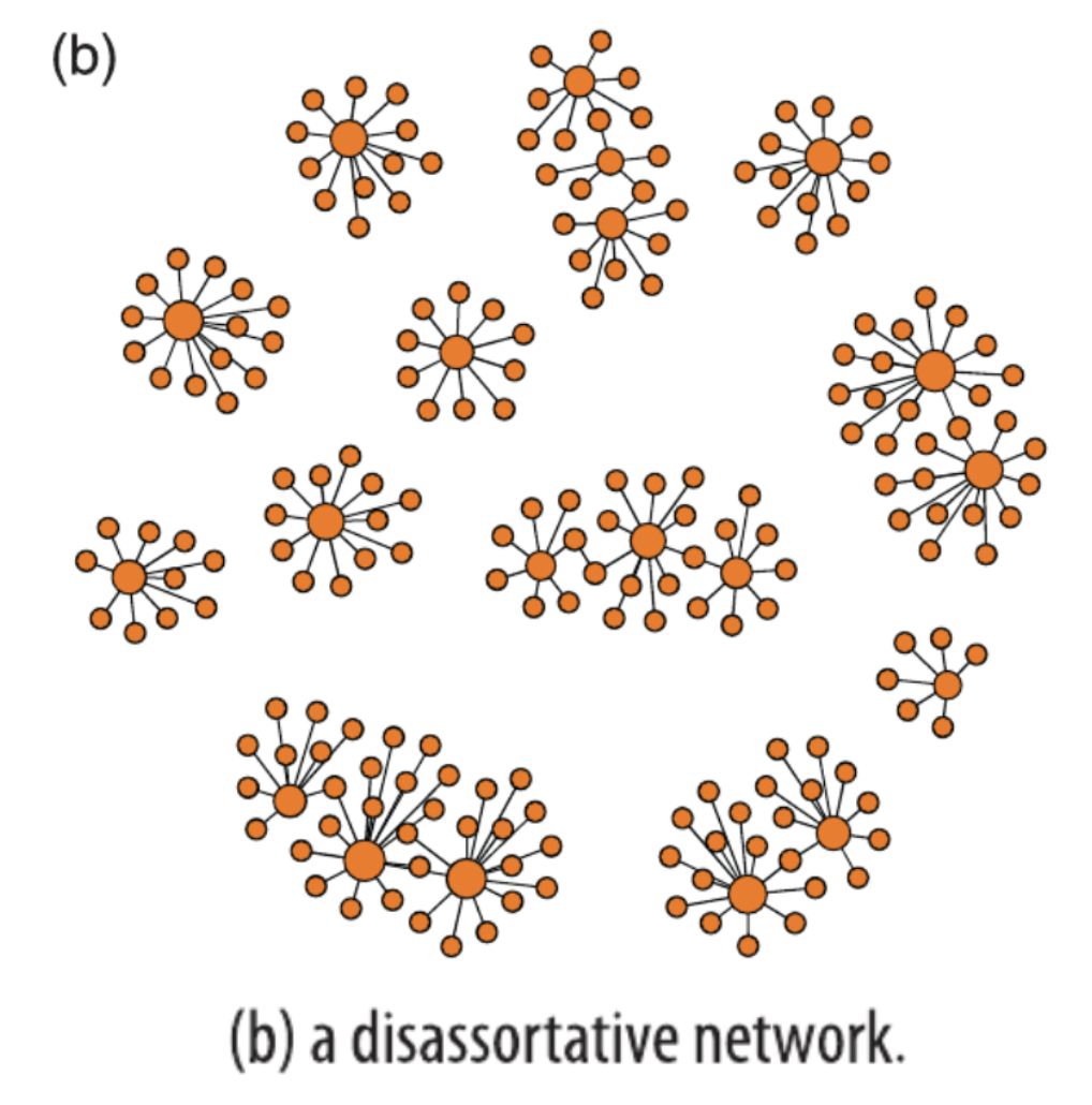
Example: Dis-assortative networks

  • This is the opposite of an assortative network, in this case, low-degree nodes tend to be connected to high-degree nodes.
  • Example: The Web, food webs, and other biological networks tend to be disassortative.
    • For example, online it is common for a low degree website to point into a high degree website via a URL.

Visualization: Comparison of assortative and disassortative networks

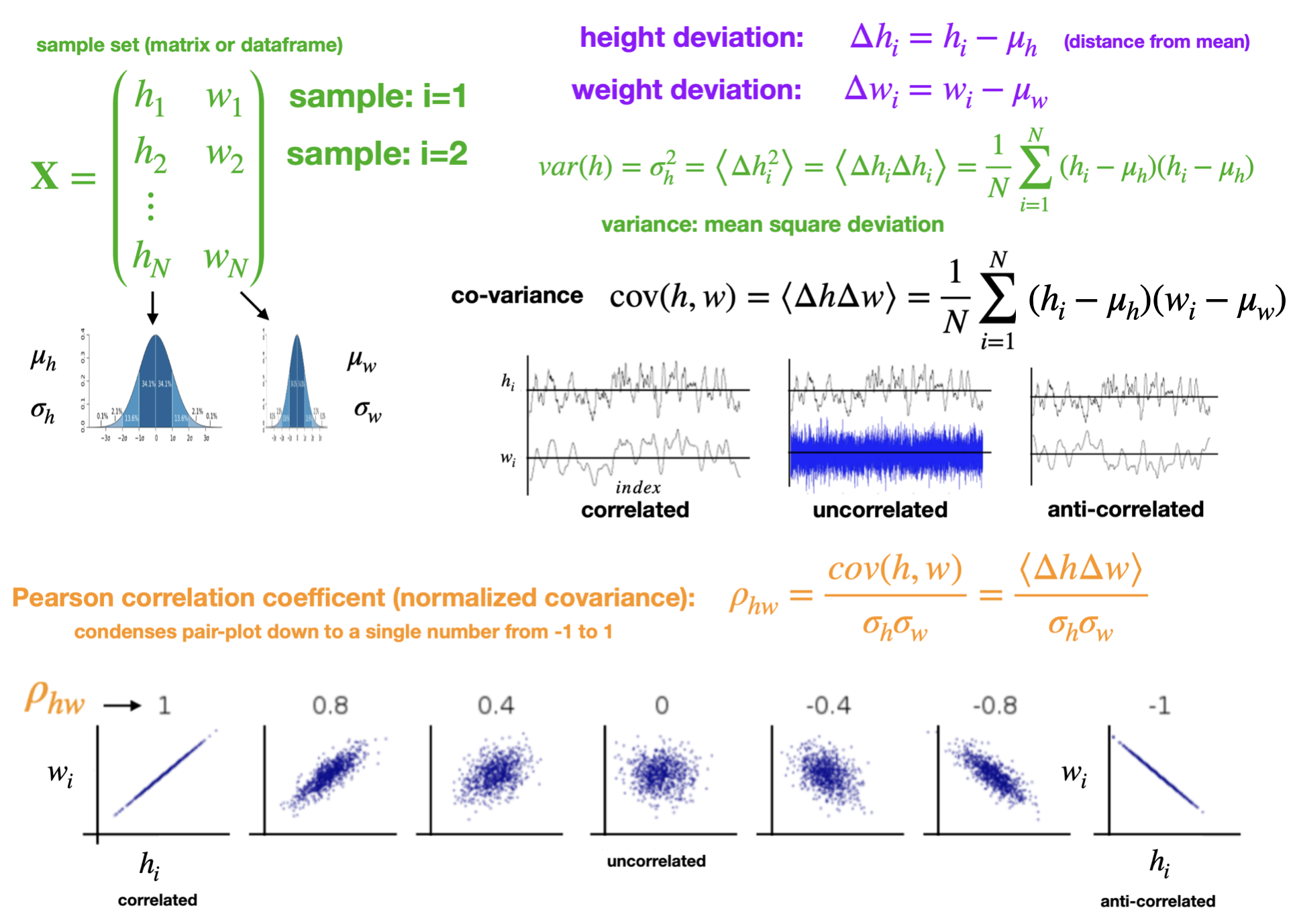
Recall: Pearson correlation

Given two vectors of equal length, you can compute the extent to which their values covary with each other
Assortativity Coefficient

  • Measures correlation between node degrees across edges
  • Specifically, the degree assortativity coefficient is a special case of the Pearson correlation coefficient

Interpretation:

  • r > 0 → Assortative: nodes tend to connect to others with similar degree
  • r = 0 → Neutral: no correlation
  • r < 0 → Disassortative: high-degree nodes connect to low-degree nodes

How it’s computed:

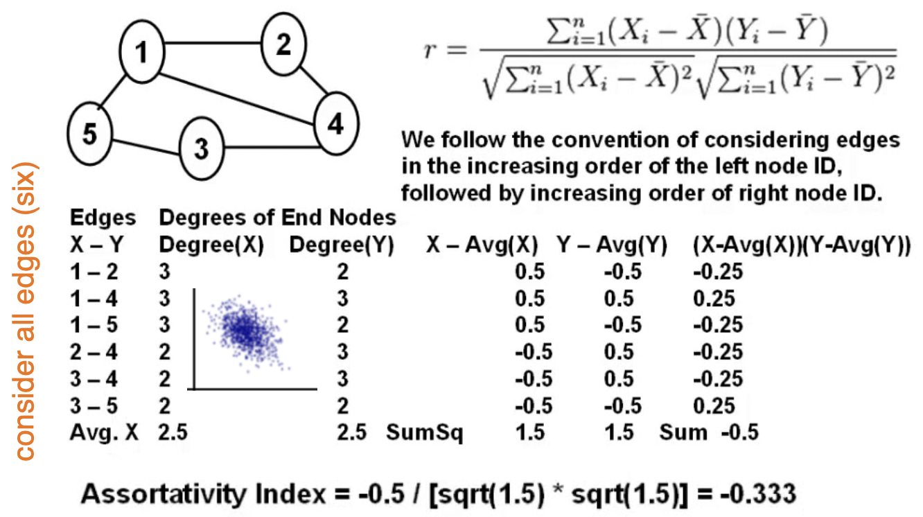
  • For each edge, define two vectors:

    • Source degrees
    • Target degrees
  • Compute Pearson correlation between these vectors

Reflects the structural tendency of a network to connect similar or dissimilar nodes.

Example: Manual Assortativity calculation

`

Example: Code Assortativity calculation

Code

import networkx as nx
import matplotlib.pyplot as plt
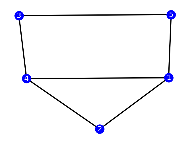
G = nx.Graph()
G.add_edges_from([(1,2),(1,4),(1,5),(2,4),(3,4),(3,5)])
nx.draw(G,
    with_labels=True,
    # labels=labels,
    node_color='blue',
    width=3,
    node_size=500,
    font_color='white',
    font_size=18,
    )

print(nx.degree_assortativity_coefficient(G)) 
-0.3333333333333304

Triangles

Triangles: Friend of a Friend

  • In a social network, if Alice and Bob are both friends of Charlie’s, then they are also likely to be friends of each other. (i.e. they form a triangle)
    • This is a three-body effect, and is a common phenomenon in social networks.
  • A triangle is a triad (set of three nodes) where each pair of nodes is connected.

Closer look at triangles

  • A triangle forms when three nodes are mutually connected (i.e., A is connected to B, B to C, and C to A)

Why Triangles Matter:

  • Represent strong local clustering
  • Capture friend-of-a-friend relationships
  • Indicate community cohesion and trust
  • Clustering Coefficient:

    • Measures how often a node’s neighbors are also connected
    • High clustering implies many local triangles
  • Transitivity:

    • Global measure of triangle density across the entire network
    • Reflects overall tendency for triadic closure

Real-World Relevance:

  • Social networks tend to form many triangles due to shared interests, mutual acquaintances, or trust reinforcement

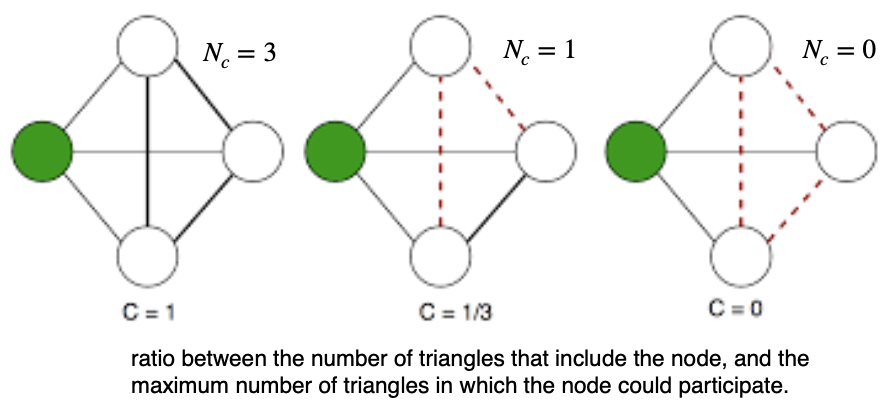
Nodal Clustering Coefficient

  • Measures how tightly connected a node’s neighbors are
  • Defined as the fraction of neighbor pairs that are connected (i.e., form triangles)

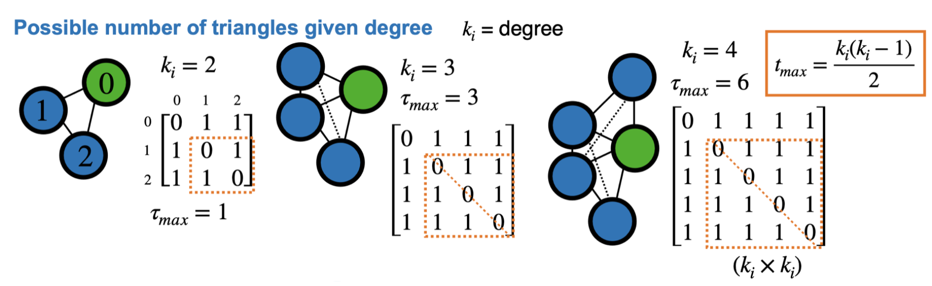
Formula:

\[ C(i) = \frac{2 \tau(i)}{k_i(k_i - 1)} \]

  • \(\tau(i)\): number of triangles involving node \(i\)
  • \(k_i\): degree of node \(i\)
  • \(\binom{k_i}{2}\): total possible neighbor pairs

\(C(i)\) is only defined for \(k_i > 1\)

Example clustering coefficient calculation

\[ C(i) = \frac{2 \tau(i)}{k_i(k_i - 1)} \]

  • \(\tau(i)\): number of triangles involving node \(i\)
  • \(k_i\): degree of node \(i\)
  • \(\binom{k_i}{2}\): total possible neighbor pairs

Network-Level Clustering Coefficient

  • Measures the overall tendency of a network to form triangles
  • High clustering (close to 1): many closed triangles (common in social networks)
  • Low clustering (close to 0): few or no triangles

Formula:

\[ C = \frac{\sum_{i: k_i > 1} C(i)}{N_{k > 1}} \]

  • Average of nodal clustering coefficients
  • Only includes nodes with degree \(k_i > 1\)

Example: Co-authorship networks often have \(C > 0.5\)

Network Connectivity

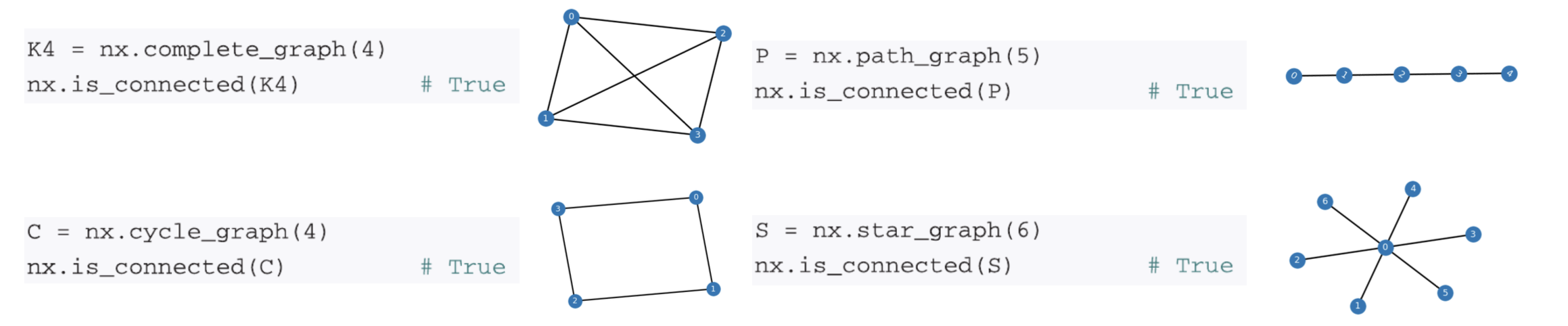
Connected Networks

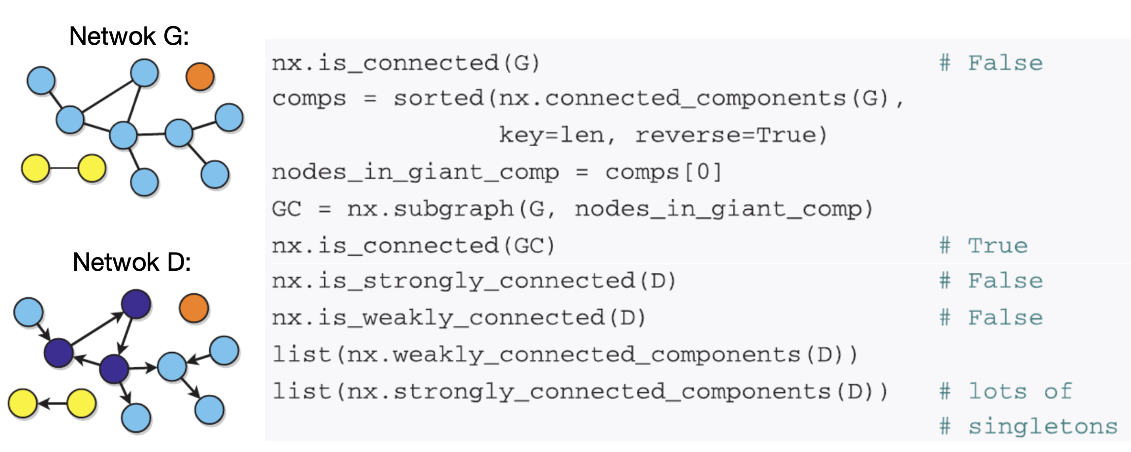
A connected network is a network where there is a path between any two nodes.

The connectedness defines many properties of a network’s physical structure.

Examples:

In NetworkX we can use the is_connected function to check if a network is connected.
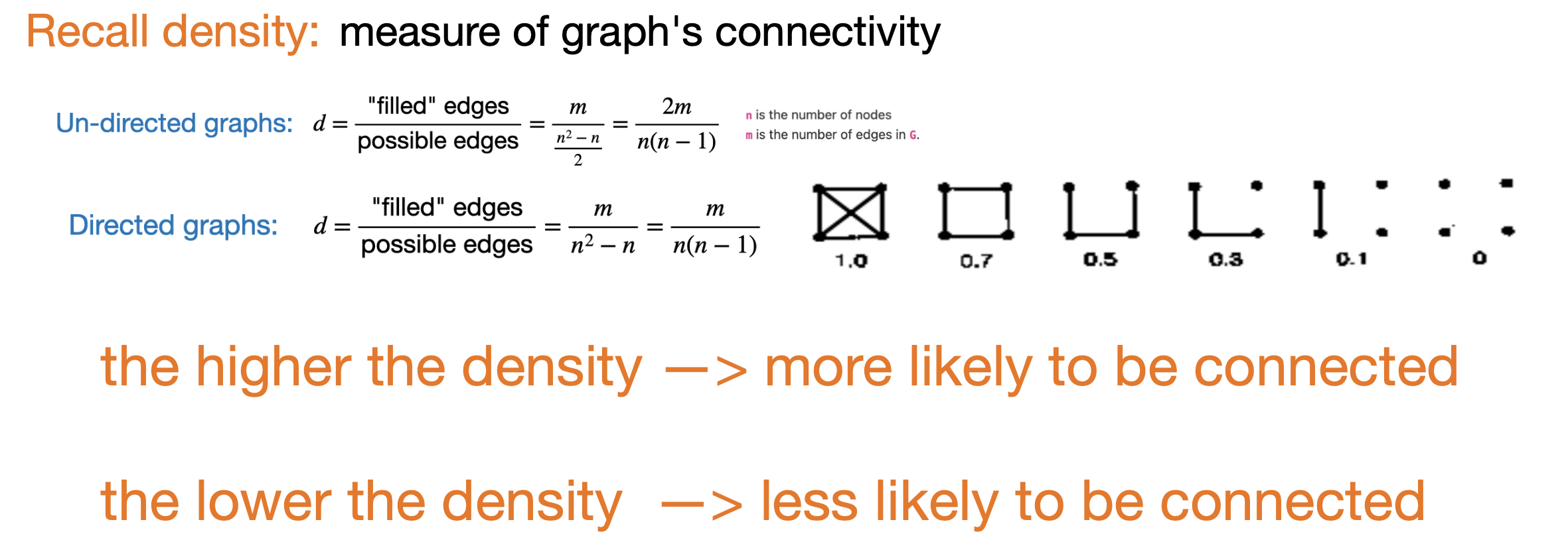
Recall Density

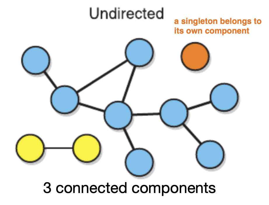
Connectedness & Components (island)

  • A disconnected network has more than one connected component (or “island”)
  • A component is a subset of nodes where every node is reachable from every other (in some sense)

Giant Connected Component (GCC):

  • The largest connected component in a network
  • In many real-world graphs, it includes a majority of nodes
  • In a fully connected network, the GCC is the entire graph

Connectedness in Directed Graphs:

In the directed case, we have to pay attention to linkdirections when determining whether a node can be reached from another.
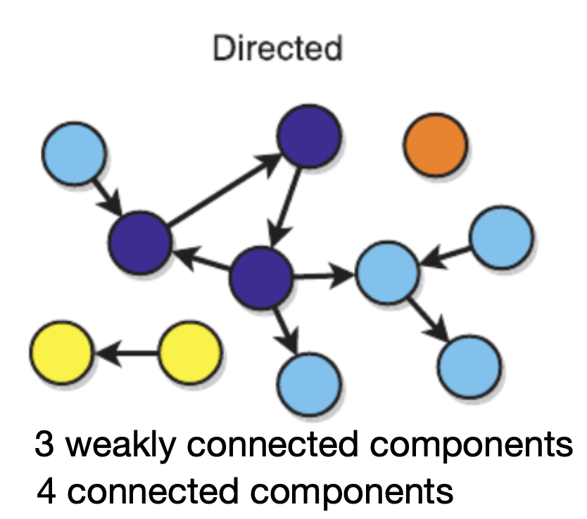
  • Weakly Connected:
    • Connectivity exists when ignoring direction of edges
  • Strongly Connected:
    • There is a directed path in both directions between every pair of nodes

NetworkX: Identifying connected components

NetworkX provides functions to identify the connected components of a network.

Distances in Disconnected Networks

  • Option 1: Focus only on nodes in the Giant Connected Component (GCC)

  • Option 2: Compute distances within each component, then average over all connected pairs

  • Diameter:

    • Calculate the diameter of each component
    • Final network diameter = maximum of all component diameters

Useful when analyzing real-world networks that are not fully connected.

Trees in Network Science

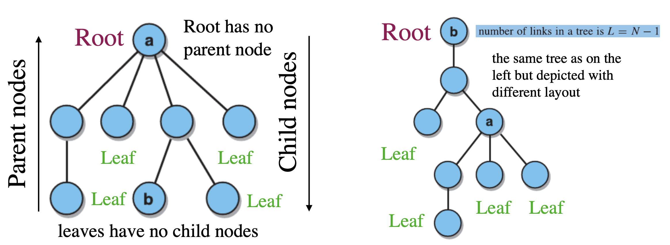
  • A tree is an undirected, connected graph with no cycles

      • No Cycles: No closed loops or circular paths
  • For \(n\) nodes, a tree has exactly \(n - 1\) edges

  • There is a unique path between any pair of nodes

  • Hierarchical: any node can be chosen as a root

  • Edge Critical:

    • Adding an edge creates a cycle
    • Removing an edge disconnects the tree

Trees are hierarchical, meaning you can pick any node in a tree to act as a root.
NetworkX has algorithms to determine whether a network is a tree.

Hubs and small worlds

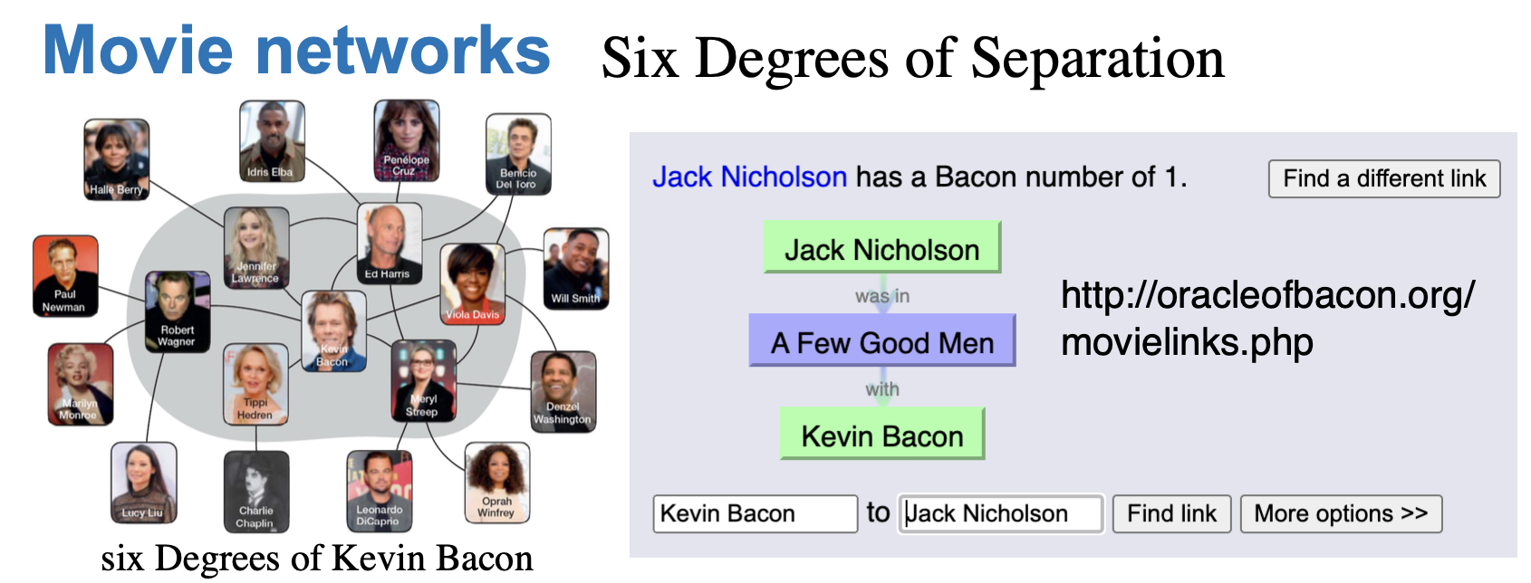
Six Degrees of Separation

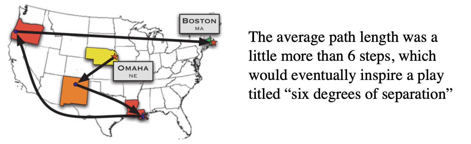
The six degrees expression arose from an experiment conducted by psychologist Stanley Milgram in the 1960s, which provided the empirical evidence of “small worlds”

Mailed letters to randomly selected individuals, asking them to forward the letter to a target person using only personal contacts

Result: Most letters reached the target in about 6 steps, giving rise to the idea of “six degrees of separation”

Small worlds phenomenon

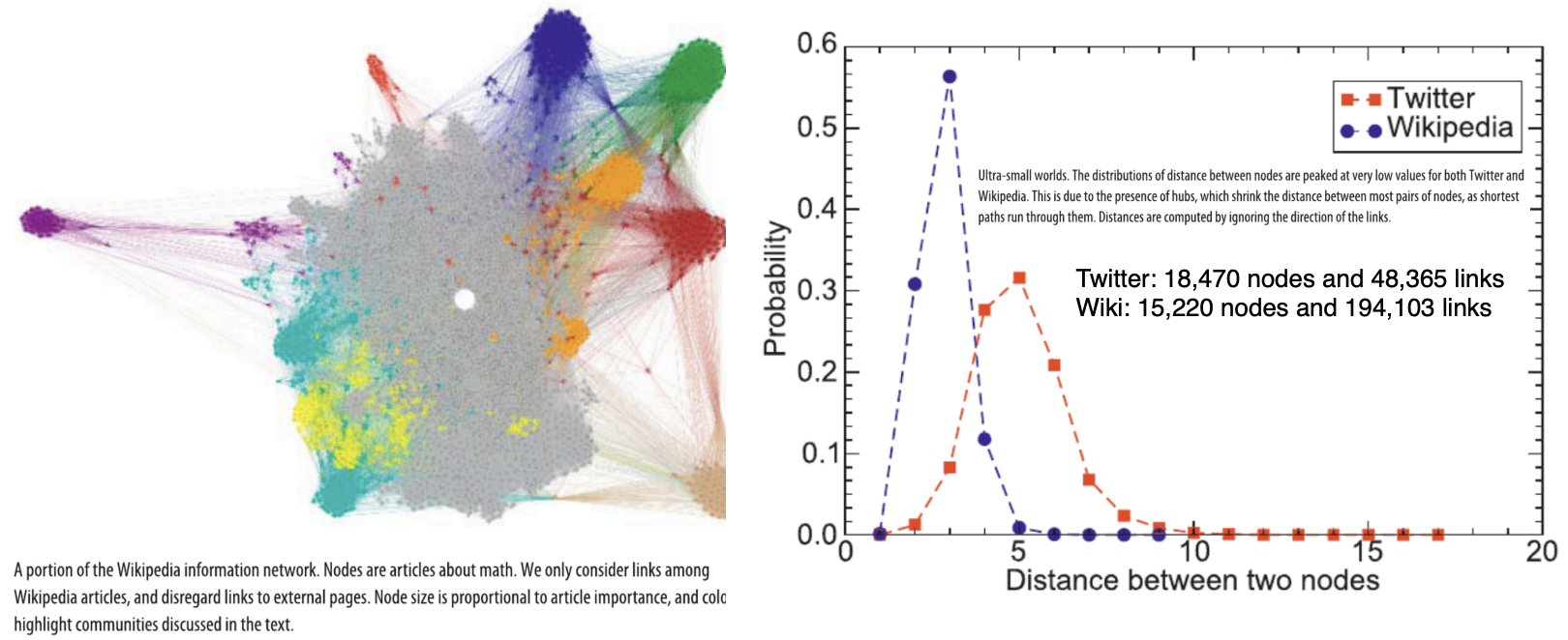
A small world network is a network where the average distance between any two nodes is small.

Most social networks have very short paths among nodes, i.e. you are likely to know someone who knows someone who knows someone…

A small world is the popular notion that social distances are short (on average)

Examples of small world networks

Co-Authorship Networks

  • A well-studied type of social collaboration network
  • Nodes: Scholars
  • Edges: Co-authored papers (data mined from digital libraries)

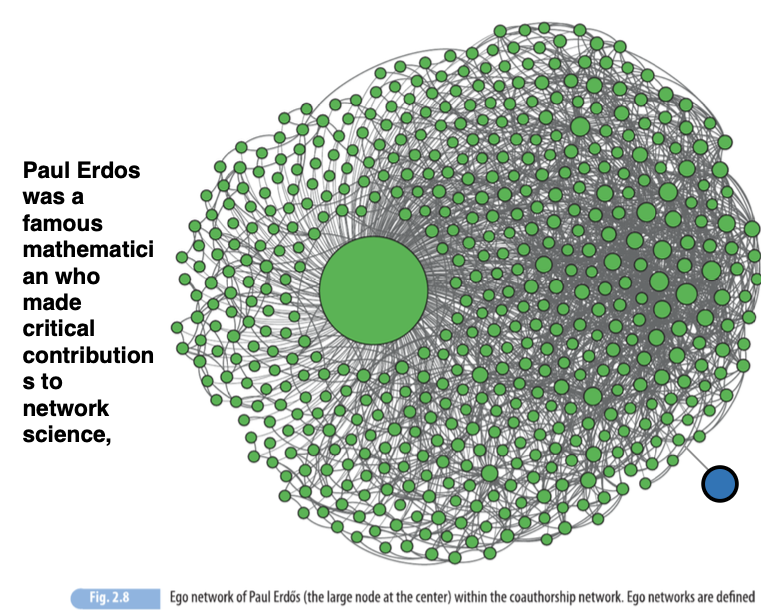
Ego Sub-Networks

  • A node (the ego) and its immediate neighbors
  • Useful for analyzing local collaboration patterns

The Erdős Number

  • Paul Erdős: prolific mathematician and central figure in co-authorship networks
  • A scholar’s Erdős number = shortest path to Erdős
  • Many scholars have low Erdős numbers, reflecting short paths in the network

Collaboration networks typically show small-world properties: short average path lengths between any two nodes

Definition of “short” depends on network size

We say that the average path length is “short” when it grows very slowly with the size of the network

We can express slow growth mathematically by saying that the average path length scales logarithmically with the size of the network:

\[ \langle\ell\rangle \sim \log N \]

The logarithm of \(a\) in base \(b, \log _b a\), is the exponent \(c\) such that \(b^c=a\). Base \(b=10\) is commonly used; \(\log _{10} 10=1\) because \(10^1=10, \log _{10} 100=2\) because \(10^2=100\), \(\log _{10} 1000=3\), etc. The logarithm is therefore a function that grows very slowly.

Hubs

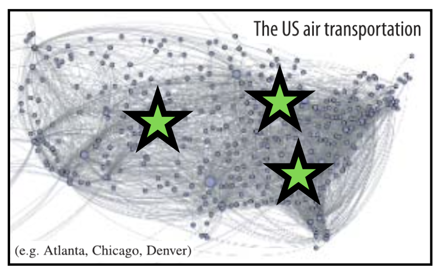
Hub: A center around which other things revolve or from which they radiate; a focus$ of activity, authority, commerce, transportation, etc.

Example:
Centrality Distributions and Heterogeneity

Recall: Centrality measures

Statistical approach

Centrality Distributions in Networks: To understand how centrality is distributed in large networks, we use statistical approaches

Why It Matters:

  • The range of the distribution reveals heterogeneity

    • Example: Node degrees spanning from 1 to millions indicate a highly heterogeneous network

Applications:

  • Helps identify sub-networks or node classes

    • Example: Group nodes by similar degree centrality
    • Focus shifts from individual nodes to patterns across the network

Centrality distributions reveal structure and inequality in node importance

Centrality distributions

A centrality distribution is the distribution of centrality values across all nodes in a network.

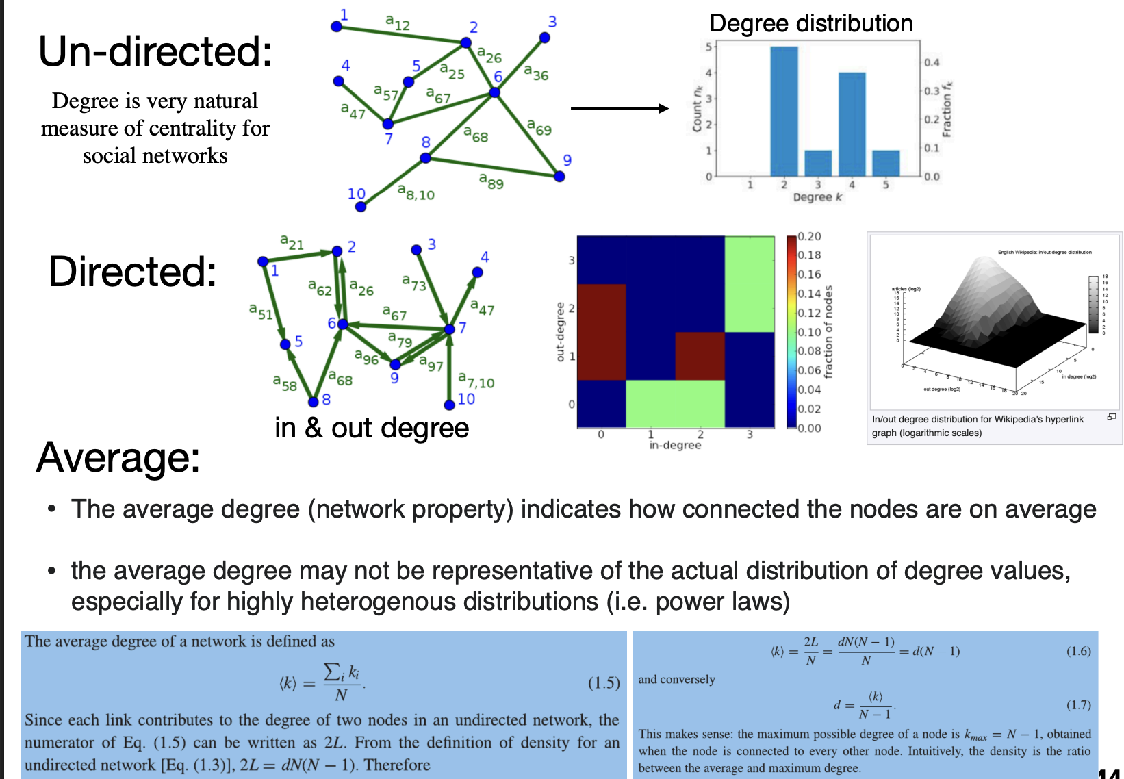
Degree distribution

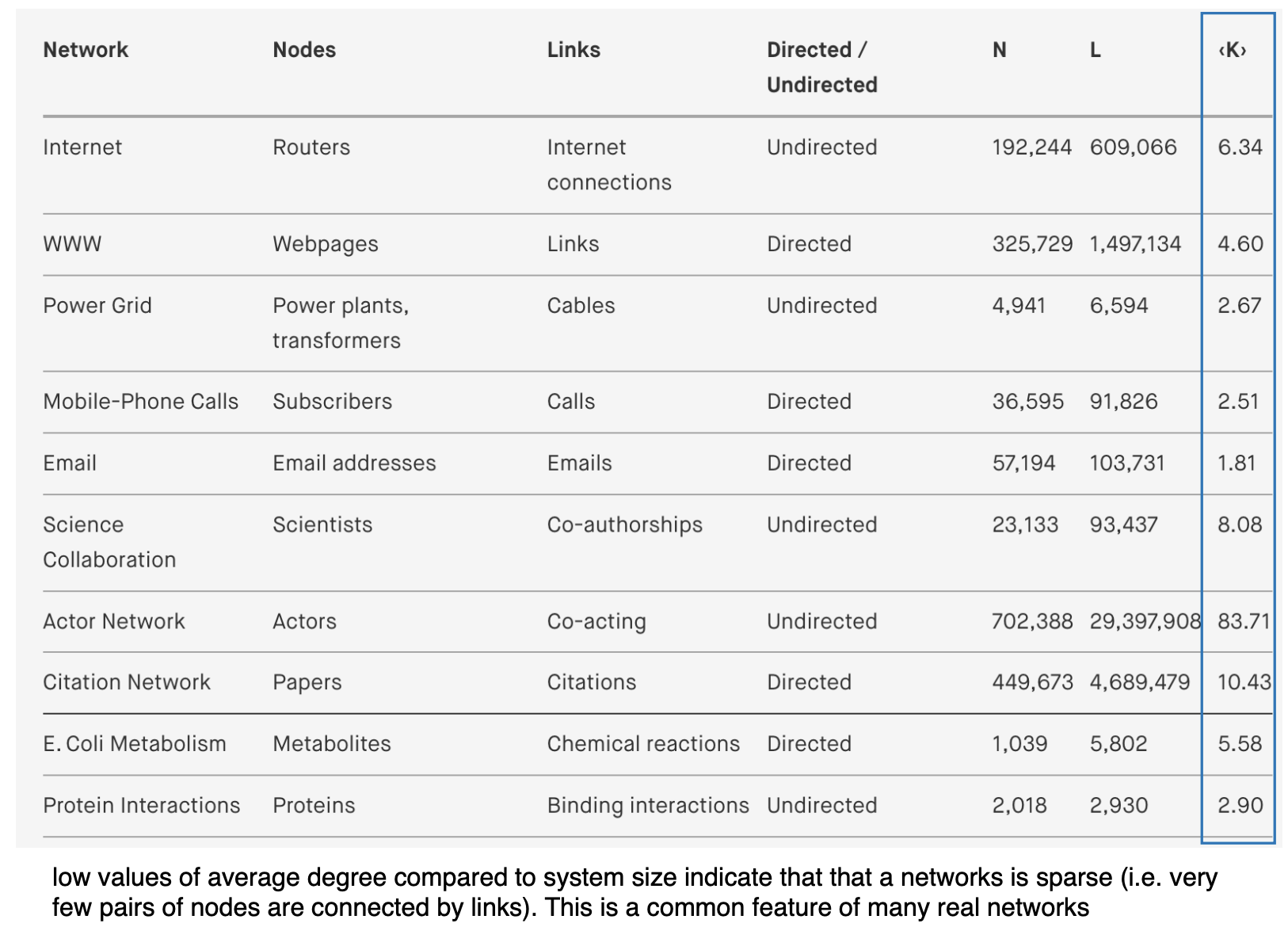
Average degree

Power-law distributions

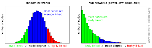
  • Many real-world networks (e.g., social, biological, internet) exhibit power law degree distributions

  • Implications:

    • Most nodes have few links, but a few have very high degree (hubs)
    • Networks are robust to random failure, but vulnerable to targeted attacks
    • Reflects self-organizing and scale-free structure

Power laws reveal the presence of inequality, hierarchy, and resilience in complex networks

Scale free (heterogenious) networks

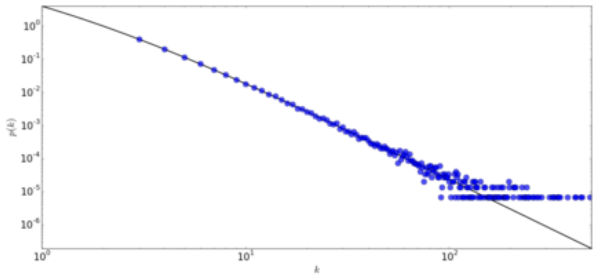
  • A scale-free network is a network whose degree distribution follows a power law, at least asymptotically.
  • That is, the fraction \(P(k)\) of nodes in the network having \(k\) connections to other nodes goes for large values of \(k\) as

\[ P(k) \sim k^{-\gamma} \]

  • where \(\gamma\) is a parameter whose value is typically in the range \(2<\gamma<3\)
  • Degree distribution for a network with 150000 vertices and mean degree created using the Barabási-Albert graph generator

Scale free networks: Video

Heterogeneity parameter

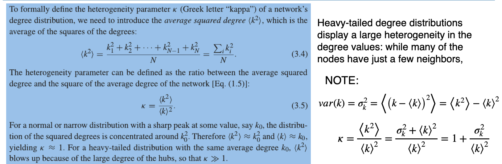
Heterogeneous networks present a wide variability in the properties and roles of their elements nodes and/or links. (Non-uniform distribution of network properties)

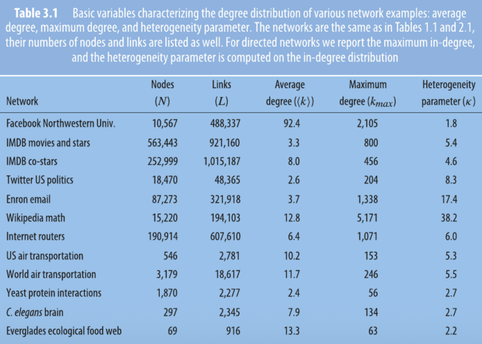
One way to measure the breadth of the degree distribution is to compute the heterogeneity parameter, which compares the variability of the degree across nodes to the average degree.
Examples

Summary

  • Assortativity measures how likely nodes are to connect to others with similar properties, such as degree or attributes, often reflecting homophily or social influence.
  • Paths are sequences of links between nodes; the shortest path defines the distance between nodes, and can be found using algorithms like breadth-first search.
  • A tree is a connected, cycle-free network with the minimum number of links.
  • Connected components are subnetworks where any two nodes are connected; in directed networks, components can be strongly or weakly connected.
  • Average path length is the mean shortest distance between all node pairs in a connected network, or within components if disconnected.
  • Small-world property describes networks where most nodes are separated by only a few steps, as in “six degrees of separation.”
  • Clustering refers to the tendency of nodes to form tightly-knit groups (triangles); the clustering coefficient quantifies this, and is typically high in social networks.