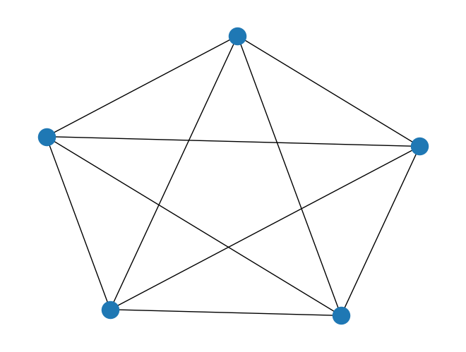
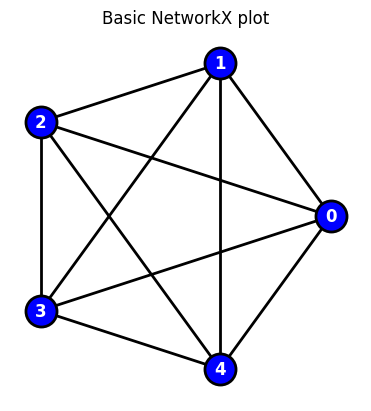
In the following self-contained example we show how to add various customization options to a plot
Code
import networkx as nximport matplotlib.pyplot as plt#GENERATE GRAPHG = nx.complete_graph(5)#BASIC PLOTnx.draw(G)plt.show()#CUSTOMIZE#specifiy x-y positions for plottingpos=nx.circular_layout(G)#initialize plotfig, ax = plt.subplots()nx.draw(G,node_color='blue',edgecolors="black",edge_color="black", linewidths=2,font_color="white",font_weight="bold",node_size=500,width=2,with_labels=True,pos=pos,ax=ax)ax.set(title='Basic NetworkX plot')ax.set_aspect('equal', 'box')#fig.savefig("test.png")plt.show()
Customizing a plot: Example-2
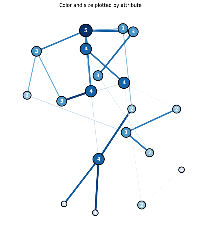
In the following self-contained example we show how to add various customization options to a NetworkX plot
Code
import networkx as nximport matplotlib.pyplot as pltimport randomimport numpy as np#GENERATE GRAPHN=20G = nx.complete_graph(N)G = nx.gnp_random_graph(N, 0.1, seed=10374196)#ASSIGN RANDOM ATTRIBUTES TO NODES+EDGESfor u in G.nodes(): G.nodes[u]['attribute']=0.2+1*random.uniform(0, 1) for u,v in G.edges(): G[u][v]['weight']=5*random.uniform(0, 1) #PRINT NODE+EDGESfor node in G.nodes(data=True): print(node)for line in nx.generate_edgelist(G, data=True): print(line)#SPECIFIY X-Y POSITIONS FOR PLOTTING# pos=nx.circular_layout(G)pos=nx.spring_layout(G,k=50*1./np.sqrt(N),iterations=500)# pos=nx.random_layout(G)#GENERATE PLOTfig, ax = plt.subplots()fig.set_size_inches(10, 10)#assign colors based on attributesweights_n = [G.nodes[u]['attribute'] for u in G.nodes()]weights_e = [G[u][v]['weight'] for u,v in G.edges()]#SAMPLE CMAP FOR COLORS cmap=plt.cm.get_cmap('Blues')colors_e = [cmap(G[u][v]['weight']/5.0) for u,v in G.edges()]colors_n = [cmap(G.nodes[u]['attribute']/1.2) for u in G.nodes()]#VARIOUS METHODS FOR VISUALIZING SIZE#LABELS (DICT)labels={}for n,d in nx.degree(G): labels[n]=d #str(n)+"-"+str(d) #WEIGHTS# node_size=1000*weights_n#DEGREE CENTRALITYcentrality=nx.degree(G)centrality=np.array([d for n,d in centrality]);#print(G_DEGREE)node_size=1000*centrality/max(centrality)colors_n = node_sizecolors_n = [cmap(u/max(centrality)) for u in centrality]#PLOTnx.draw(G, node_color=colors_n, edgecolors="black", edge_color=colors_e, linewidths=2, labels=labels, font_color="white", font_weight="bold", node_size=node_size, width=weights_e, with_labels=True, pos=pos, ax=ax)#TITLE ax.set(title='Color and size plotted by attribute')ax.set_aspect('equal', 'box')#PLOT# fig.savefig("test.png")plt.show()
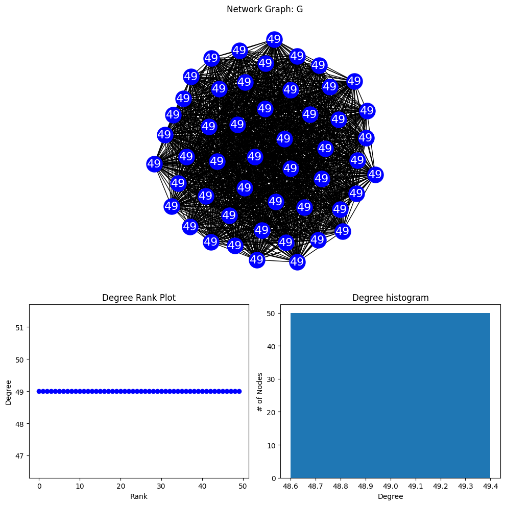
NETWORK DENSITY: 1.0
 NETWORK DIAMETER: 1

BINOMIAL TREE
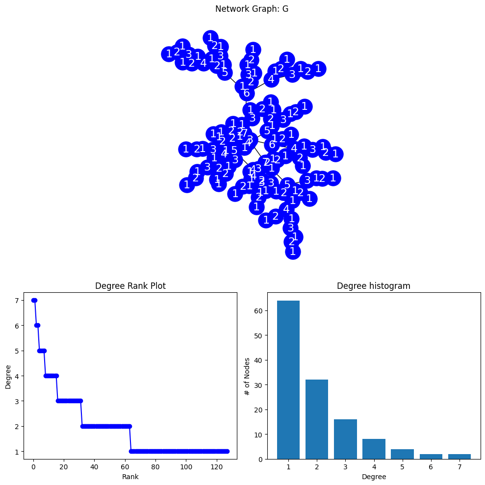
NETWORK DENSITY: 0.015625
 NETWORK DIAMETER: 13
Graph Layouts
A graph visualization layout arranges nodes and edges in a visually intuitive manner.
Examples include hierarchical trees with parent-child relationships, force-directed layouts where nodes repel each other, and circular layouts that arrange nodes in a circle.
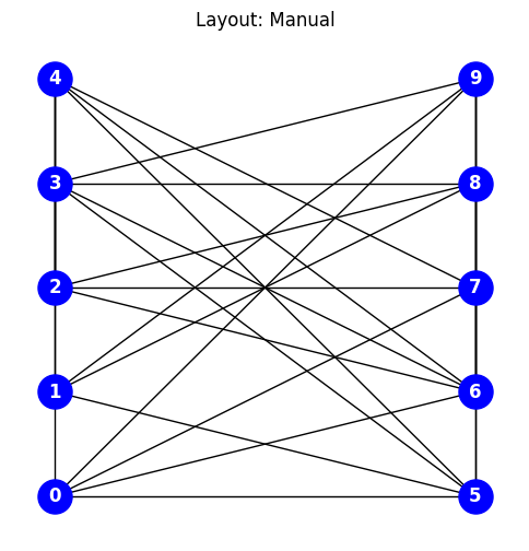
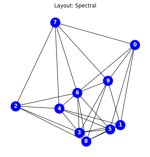
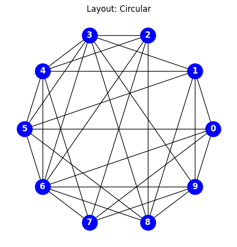
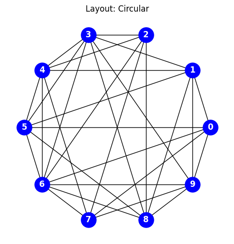
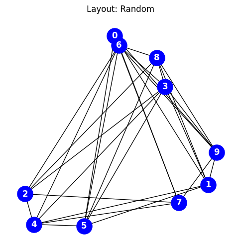
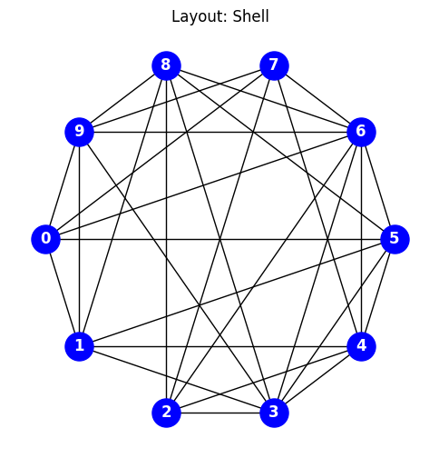
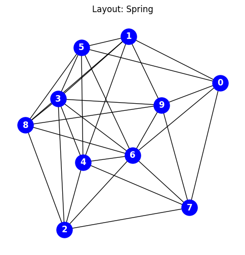
In the following example the code explores various Network-X positional layouts
Code
import networkx as nximport matplotlib.pyplot as plt#GENERATE A COMPLETE GRAPH USING A GRAPH GENERATOR #https://networkx.org/documentation/stable/reference/generators.html# G = nx.complete_graph(10)G = nx.gnp_random_graph(10,p=0.7)for i inrange(1,7+1):#print(i)#CAN MANUALLY SPECIFY GRAPH LOCATIONS WITH A DICTIONARY OF (X,Y) ARRAYS if(i==1): title="Layout: Manual"; pos={}; j=0; i1=0for k inrange(0,len(list(G.edges))):if(k%5==0): j=j+1if(k%5==0): i1=0 i1=i1+1 pos[k]=[j,i1]# OR YOU CAN USE ONE OF NETWORK-X'S BUILT-IN POSITION LAYOUT ALGORITHMSif(i==2): title="Layout: Spectral"; pos = nx.spectral_layout(G)if(i==3): title="Layout: Circular"; pos = nx.circular_layout(G)# if(i==4): title="Layout: Kamada-Kawai"; pos = nx.kamada_kawai_layout(G)if(i==5): title="Layout: Random"; pos = nx.random_layout(G)if(i==6): title="Layout: Shell"; pos = nx.shell_layout(G)if(i==7): title="Layout: Spring"; pos = nx.spring_layout(G,iterations=200) fig, ax = plt.subplots() fig.set_size_inches(6, 6) nx.draw( G, node_color="blue", node_size=500, font_color="white", font_weight="bold", with_labels=True, pos=pos, ) ax.set(title=title)# if(i>1): ax.set_aspect('equal', 'box') plt.title(title) plt.show()