['A', 1]
<class 'str'>
<class 'int'>Introduction to NetworkX
This notebook provides a practical and conceptual introduction to the Python library NetworkX, one of the most widely used frameworks for graph and network analysis.
Topics covered include:
- Graph theory fundamentals
- Creating graphs
- Adding nodes and edges
- Graph visualization
- Directed and weighted graphs
- Network statistics and metrics
- Centrality measures
- Community detection concepts
- Real-world style network examples
- Exporting and importing graphs
NetworkX: Comprehensive Package Overview
NetworkX is a Python library for the creation, manipulation, and study of complex networks (graphs). It provides data structures for graphs, digraphs, and multigraphs along with a large suite of algorithms for graph analysis.
networkx/
├── classes/          # Core graph classes (Graph, DiGraph, MultiGraph, MultiDiGraph)
├── algorithms/       # All graph algorithms (>30 sub-modules)
│   ├── shortest_paths/
│   ├── traversal/
│   ├── connectivity/
│   ├── flow/
│   ├── centrality/
│   ├── community/
│   ├── isomorphism/
│   ├── approximation/
│   ├── bipartite/
│   └── ...
├── generators/       # Graph generator functions
│   ├── classic/
│   ├── random_graphs/
│   ├── lattice/
│   ├── community/
│   └── ...
├── readwrite/        # I/O for various formats
├── drawing/          # Visualization (matplotlib, graphviz)
├── convert/          # Format conversions
├── linalg/           # Matrix / spectral functions
└── utils/            # Shared utilities and decorators
1. Core Data Structures
NetworkX provides four primary graph classes, each representing a different type of network.
1.1 Graph (Undirected)
- Edges have no direction;
(u, v)and(v, u)are the same edge. - Self-loops are allowed.
- No parallel (duplicate) edges between the same pair of nodes.
- Key use cases: social networks, physical infrastructure, molecule modeling.
1.2 DiGraph (Directed)
- Edges have direction;
(u, v)and(v, u)are distinct. - Supports in-degree / out-degree and predecessor / successor queries.
- Key use cases: dependency graphs, web link graphs, control flow.
1.3 MultiGraph (Undirected, Parallel Edges)
- Undirected graph that allows multiple edges between the same pair of nodes.
- Each parallel edge has a unique integer key.
- Key use cases: transportation networks where multiple routes exist.
1.4 MultiDiGraph (Directed, Parallel Edges)
- Directed graph with parallel edge support.
- Combines the properties of
DiGraphandMultiGraph. - Key use cases: citation networks with multiple relationship types.
1.5 Internal Data Model
- Nodes and edges are stored in nested dictionaries (
dict-of-dict-of-dict). - Nodes are any hashable Python object (int, str, tuple, frozen sets, etc.).
- Edges can carry arbitrary attribute dictionaries.
- Adjacency represented via
G._adj(outer: source node, inner: neighbor, innermost: edge data).
2. Graph Construction & Manipulation
2.1 Adding Nodes
| Method | Description |
|---|---|
G.add_node(n, **attr) |
Add a single node with optional attributes |
G.add_nodes_from(nodes) |
Add nodes from any iterable |
G.remove_node(n) |
Remove node and all incident edges |
G.remove_nodes_from(nodes) |
Remove multiple nodes |
G.clear() |
Remove all nodes and edges |
2.2 Adding Edges
| Method | Description |
|---|---|
G.add_edge(u, v, **attr) |
Add a single edge with optional attributes |
G.add_edges_from(ebunch) |
Add edges from iterable of (u, v) or (u, v, data) |
G.add_weighted_edges_from(ebunch) |
Add edges with a weight attribute |
G.remove_edge(u, v) |
Remove edge between u and v |
G.remove_edges_from(ebunch) |
Remove multiple edges |
G.update(edges, nodes) |
Update graph from edges and/or nodes |
2.3 Graph-Level Properties
| Property / Method | Description |
|---|---|
G.number_of_nodes() |
Count of nodes |
G.number_of_edges() |
Count of edges |
G.order() |
Alias for number of nodes |
G.size(weight=None) |
Total edges (or total weight if weight given) |
G.is_directed() |
Returns True for DiGraph / MultiDiGraph |
G.is_multigraph() |
Returns True for MultiGraph / MultiDiGraph |
G.graph |
Dictionary of graph-level attributes |
3. Node & Edge Attributes
3.1 Node Attributes
- Stored as a dictionary on each node:
G.nodes[n]. - Set via
G.add_node(n, color='red')orG.nodes[n]['color'] = 'red'. G.nodesreturns aNodeViewsupporting iteration, membership, and data access.G.nodes(data=True)yields(node, attr_dict)tuples.G.nodes(data='weight', default=1.0)yields(node, value)for a single attribute.
3.2 Edge Attributes
- Stored as a dictionary per edge:
G.edges[u, v]. - Common attributes:
weight,capacity,label,color, etc. G.edgesreturns anEdgeView.G.edges(data=True)yields(u, v, attr_dict)tuples.G.edges(data='weight', default=1)yields(u, v, value).
3.3 Degree Views
| Method | Description |
|---|---|
G.degree() |
DegreeView of all nodes |
G.degree(weight='weight') |
Weighted degree (sum of edge weights) |
DG.in_degree() |
In-degree for directed graphs |
DG.out_degree() |
Out-degree for directed graphs |
4. Graph Generators
NetworkX ships hundreds of built-in generators across multiple categories.
4.1 Classic Graphs
nx.complete_graph(n)— fully connected graph \(K_n\)nx.path_graph(n)— linear chainnx.cycle_graph(n)— closed cyclenx.star_graph(n)— hub-and-spokenx.wheel_graph(n)— cycle plus central hubnx.empty_graph(n)— n nodes, no edgesnx.null_graph()— empty graph (no nodes)nx.trivial_graph()— single nodenx.petersen_graph(),nx.dodecahedral_graph(), etc. — named graphs
4.2 Random Graphs
nx.erdos_renyi_graph(n, p)— Erdős–Rényi \(G(n, p)\) modelnx.gnm_random_graph(n, m)— \(G(n, m)\) random graph with exactly m edgesnx.barabasi_albert_graph(n, m)— preferential attachment (scale-free)nx.watts_strogatz_graph(n, k, p)— small-world modelnx.newman_watts_strogatz_graph(n, k, p)— variant small-worldnx.random_regular_graph(d, n)— d-regular random graphnx.powerlaw_cluster_graph(n, m, p)— power-law with clusteringnx.random_lobster(n, p1, p2)— lobster structurenx.random_tree(n)— random labeled tree
4.3 Lattice & Grid Graphs
nx.grid_graph(dim)— n-dimensional gridnx.grid_2d_graph(m, n)— rectangular 2D gridnx.hexagonal_lattice_graph(m, n)— honeycomb latticenx.triangular_lattice_graph(m, n)— triangular tilingnx.hypercube_graph(n)— n-dimensional hypercube
4.4 Social & Community Graphs
nx.karate_club_graph()— Zachary’s karate club (classic benchmark)nx.florentine_families_graph()— Renaissance Florence marriagesnx.davis_southern_women_graph()— bipartite social networknx.les_miserables_graph()— co-occurrence network
4.5 Tree Generators
nx.balanced_tree(r, h)— complete r-ary tree of height hnx.full_rary_tree(r, n)— r-ary tree with n nodesnx.random_tree(n)— uniform random labeled treenx.prefix_tree(paths)— trie from iterable of paths
4.6 Directed Graph Generators
nx.gn_graph(n)— growing network (directed)nx.gnr_graph(n, p)— growing network with redirectionnx.gnc_graph(n)— growing network with copyingnx.scale_free_graph(n)— scale-free directed graphnx.random_k_out_graph(n, k, alpha)— random k-out graph
4.7 Bipartite Graph Generators
nx.bipartite.complete_bipartite_graph(n1, n2)— \(K_{n1,n2}\)nx.bipartite.random_graph(n, m, p)— random bipartitenx.bipartite.gnmk_random_graph(n, m, k)— bipartite with k edgesnx.bipartite.configuration_model(aseq, bseq)— degree sequence model
4.8 Geometric / Spatial Graphs
nx.random_geometric_graph(n, radius)— nodes in unit square, edges by proximitynx.waxman_graph(n, beta, alpha)— probability decays with distancenx.geographical_threshold_graph(n, theta)— threshold-based spatial graphnx.soft_random_geometric_graph(n, radius)— soft version of geometric graph
4.9 Intersection Graphs
nx.uniform_random_intersection_graph(n, m, p)— random intersectionnx.k_random_intersection_graph(n, m, k)— k-random intersection
4.10 Spectral / Algebraic Graphs
nx.margulis_gabber_galil_graph(n)— Ramanujan expandernx.chordal_cycle_graph(p)— chordal cycle
5. Graph Input / Output (I/O)
NetworkX can read and write graphs in many standard formats.
5.1 Adjacency / Edge List Formats
| Function | Description |
|---|---|
nx.read_edgelist(path) |
Read edge list (space-separated) |
nx.write_edgelist(G, path) |
Write edge list |
nx.read_adjlist(path) |
Read adjacency list |
nx.write_adjlist(G, path) |
Write adjacency list |
nx.read_weighted_edgelist(path) |
Edge list with weights |
nx.write_weighted_edgelist(G, path) |
Write with weights |
5.2 GML / GraphML / GEXF
| Function | Description |
|---|---|
nx.read_gml(path) |
Read Graph Markup Language file |
nx.write_gml(G, path) |
Write GML |
nx.read_graphml(path) |
Read GraphML (XML-based) |
nx.write_graphml(G, path) |
Write GraphML |
nx.read_gexf(path) |
Read GEXF (Gephi format) |
nx.write_gexf(G, path) |
Write GEXF |
5.3 Pickle & JSON
| Function | Description |
|---|---|
nx.read_gpickle(path) |
Read Python pickle |
nx.write_gpickle(G, path) |
Write Python pickle |
nx.node_link_data(G) |
Convert to node-link dict (JSON-friendly) |
nx.node_link_graph(data) |
Restore from node-link dict |
nx.adjacency_data(G) |
Adjacency-list JSON representation |
nx.adjacency_graph(data) |
Restore from adjacency dict |
nx.tree_data(G, root) |
Serialize tree as nested dict |
nx.tree_graph(data) |
Restore tree from dict |
5.4 Matrix / SciPy Formats
| Function | Description |
|---|---|
nx.to_numpy_array(G) |
Dense adjacency matrix (NumPy) |
nx.from_numpy_array(A) |
Graph from dense matrix |
nx.to_scipy_sparse_array(G) |
Sparse adjacency matrix |
nx.from_scipy_sparse_array(A) |
Graph from sparse matrix |
nx.to_pandas_adjacency(G) |
Adjacency DataFrame |
nx.from_pandas_adjacency(df) |
Graph from adjacency DataFrame |
nx.to_pandas_edgelist(G) |
Edge list DataFrame |
nx.from_pandas_edgelist(df) |
Graph from edge DataFrame |
5.5 Specialized Formats
| Function | Description |
|---|---|
nx.read_pajek(path) |
Pajek network format |
nx.write_pajek(G, path) |
Write Pajek |
nx.read_leda(path) |
LEDA native format |
nx.read_multiline_adjlist(path) |
Multiline adjacency list |
nx.write_multiline_adjlist(G, path) |
Write multiline adj list |
6. Algorithms
This is the largest and most comprehensive part of NetworkX.
6.1 Shortest Paths
6.1.1 Unweighted (BFS-based)
nx.shortest_path(G, source, target)— single pairnx.shortest_path_length(G, source, target)— hop countnx.all_shortest_paths(G, source, target)— all shortest pathsnx.single_source_shortest_path(G, source)— from one source to allnx.all_pairs_shortest_path(G)— all pairsnx.all_pairs_shortest_path_length(G)— all pairs lengths
6.1.2 Weighted (Dijkstra)
nx.dijkstra_path(G, source, target, weight)— optimal single-pair pathnx.dijkstra_path_length(G, source, target, weight)— path costnx.single_source_dijkstra(G, source)— distances from one sourcenx.all_pairs_dijkstra(G)— all-pairs Dijkstranx.multi_source_dijkstra(G, sources)— multiple simultaneous sources
6.1.3 Bellman-Ford & Floyd-Warshall
nx.bellman_ford_path(G, source, target)— handles negative weightsnx.single_source_bellman_ford(G, source)— from one sourcenx.floyd_warshall(G)— dense all-pairs dictionarynx.floyd_warshall_numpy(G)— returns NumPy matrixnx.floyd_warshall_predecessor_and_distance(G)— with predecessor map
6.1.4 A* Search
nx.astar_path(G, source, target, heuristic)— heuristic-guided shortest pathnx.astar_path_length(G, source, target, heuristic)— path cost
6.2 Traversal
6.2.1 Breadth-First Search (BFS)
nx.bfs_edges(G, source)— edges in BFS ordernx.bfs_tree(G, source)— BFS spanning treenx.bfs_predecessors(G, source)— predecessor mappingnx.bfs_successors(G, source)— successors at each levelnx.bfs_layers(G, sources)— nodes grouped by BFS depthnx.descendants_at_distance(G, source, distance)— nodes at exact BFS depth
6.2.2 Depth-First Search (DFS)
nx.dfs_edges(G, source)— edges in DFS ordernx.dfs_tree(G, source)— DFS spanning treenx.dfs_predecessors(G, source)— DFS predecessor mapnx.dfs_successors(G, source)— DFS successorsnx.dfs_preorder_nodes(G, source)— nodes in DFS pre-ordernx.dfs_postorder_nodes(G, source)— nodes in DFS post-order
6.3 Connectivity
6.3.1 Undirected Connectivity
nx.is_connected(G)— single connected component checknx.number_connected_components(G)— count componentsnx.connected_components(G)— generator of component node setsnx.node_connected_component(G, n)— component containing node nnx.is_biconnected(G)— biconnectivity checknx.biconnected_components(G)— biconnected component setsnx.articulation_points(G)— nodes whose removal disconnects graphnx.bridges(G)— edges whose removal disconnects graph
6.3.2 Directed Connectivity
nx.is_weakly_connected(DG)— weakly connected checknx.is_strongly_connected(DG)— strongly connected checknx.is_semiconnected(DG)— semiconnected checknx.strongly_connected_components(DG)— Tarjan / Kosaraju SCCsnx.weakly_connected_components(DG)— weakly connected componentsnx.condensation(DG)— DAG of SCCs
6.3.3 Node & Edge Connectivity (Flow-based)
nx.node_connectivity(G, s, t)— min nodes to disconnect s from tnx.edge_connectivity(G, s, t)— min edges to disconnect s from tnx.minimum_node_cut(G, s, t)— minimum node cut setnx.minimum_edge_cut(G, s, t)— minimum edge cut setnx.all_node_cuts(G)— all minimum node cutsnx.stoer_wagner(G)— global minimum cut (undirected, Stoer-Wagner)
6.4 Flow Algorithms
nx.maximum_flow(G, s, t)— Edmonds-Karp max flownx.maximum_flow_value(G, s, t)— only the flow valuenx.minimum_cut(G, s, t)— min cut (value + partition)nx.minimum_cut_value(G, s, t)— only the cut valuenx.min_cost_flow(G)— minimum cost flow on capacitated graphnx.min_cost_flow_cost(G)— total cost of min-cost flownx.max_flow_min_cost(G, s, t)— maximum flow at minimum costnx.network_simplex(G)— network simplex algorithmnx.capacity_scaling(G)— capacity scaling algorithm
6.5 Centrality Measures
| Function | Description |
|---|---|
nx.degree_centrality(G) |
Normalized degree per node |
nx.betweenness_centrality(G) |
Fraction of shortest paths through node |
nx.edge_betweenness_centrality(G) |
Betweenness for edges |
nx.closeness_centrality(G) |
Inverse average shortest path |
nx.eigenvector_centrality(G) |
Influence via neighbor influence |
nx.pagerank(G, alpha) |
Google PageRank |
nx.hits(G) |
Hyperlink-Induced Topic Search (hubs & authorities) |
nx.katz_centrality(G, alpha) |
Attenuation-weighted walk count |
nx.load_centrality(G) |
Load-based centrality |
nx.harmonic_centrality(G) |
Sum of inverse distances |
nx.voterank(G) |
VoteRank iterative ranking |
nx.percolation_centrality(G) |
Centrality based on percolation state |
nx.second_order_centrality(G) |
Standard deviation of return times |
6.6 Clustering
nx.clustering(G, nodes, weight)— clustering coefficient per nodenx.average_clustering(G)— mean clustering coefficientnx.transitivity(G)— global clustering coefficientnx.triangles(G)— triangle count per nodenx.generalized_degree(G)— number of triangles for each node pairnx.square_clustering(G)— 4-cycle ratio (bipartite-friendly)
6.7 Community Detection
nx.community.greedy_modularity_communities(G)— greedy modularity maximization (CNM)nx.community.louvain_communities(G)— Louvain methodnx.community.girvan_newman(G)— edge betweenness hierarchical splittingnx.community.label_propagation_communities(G)— LPAnx.community.asyn_lpa_communities(G)— asynchronous LPAnx.community.k_clique_communities(G, k)— clique percolation methodnx.community.modularity(G, communities)— compute modularity Qnx.community.coverage(G, communities)— fraction of edges within communitiesnx.community.performance(G, communities)— performance metricnx.community.partition_quality(G, communities)— coverage + performance
6.8 Cliques
nx.find_cliques(G)— all maximal cliques (Bron–Kerbosch)nx.clique_number(G)— size of largest cliquenx.graph_clique_number(G)— aliasnx.node_clique_number(G)— clique number for each nodenx.cliques_containing_node(G, v)— cliques involving a nodenx.make_clique_bipartite(G)— clique-node bipartite graphnx.enumerate_all_cliques(G)— all cliques, not just maximal
6.9 Spanning Trees & Forests
nx.minimum_spanning_tree(G, weight, algorithm)— MST (Kruskal / Prim / Borůvka)nx.maximum_spanning_tree(G, weight, algorithm)— maximum weight spanning treenx.minimum_spanning_edges(G)— MST edge generatornx.maximum_spanning_edges(G)— max spanning edge generatornx.minimum_spanning_forest(G)— MST/forest for disconnected graphsnx.number_of_spanning_trees(G)— count via Kirchhoff’s matrix tree theorem
6.10 Tree Algorithms
nx.is_tree(G)— is graph a tree?nx.is_forest(G)— is graph a forest?nx.is_arborescence(G)— directed rooted tree?nx.is_branching(G)— directed forest?nx.topological_sort(G)— linear ordering of DAG nodesnx.topological_generations(G)— nodes grouped by topological levelnx.lexicographic_topological_sort(G)— topo sort with tie-breakingnx.is_directed_acyclic_graph(G)— DAG checknx.ancestors(G, source)— all ancestors in DAGnx.descendants(G, source)— all descendants in DAGnx.dag_longest_path(G)— critical path in DAGnx.dag_longest_path_length(G)— length of critical pathnx.transitive_closure(G)— reachability graphnx.transitive_reduction(G)— minimal equivalent DAG
6.11 Matching
nx.max_weight_matching(G)— maximum weight matching (general graphs)nx.maximum_matching(G)— maximum cardinality matchingnx.is_perfect_matching(G, matching)— validates perfect matchingnx.min_weight_matching(G)— minimum weight matching- Bipartite matching:
nx.bipartite.maximum_matching(B)— Hopcroft-Karp for bipartitenx.bipartite.minimum_weight_full_matching(B)— min weight bipartitenx.bipartite.eppstein_matching(B)— Eppstein’s algorithm
6.12 Graph Isomorphism
nx.is_isomorphic(G1, G2)— graph isomorphism test (VF2)nx.is_subgraph_isomorphic(G1, G2)— subgraph isomorphismnx.graph_edit_distance(G1, G2)— minimum edit distancenx.optimal_edit_paths(G1, G2)— all optimal edit sequencesnx.GraphMatcher(G1, G2)— iterative isomorphism matchernx.DiGraphMatcher(G1, G2)— directed versionnx.vf2userfunc.GMState/DiGMState— internal VF2 state objects
6.13 Planarity
nx.is_planar(G)— planarity test (LR-planarity / Boyer-Myrvold)nx.check_planarity(G)— returns(is_planar, embedding)nx.PlanarEmbedding— combinatorial planar embedding objectnx.is_bipartite(G)— check if graph is bipartite (planarity-related)
6.14 Coloring
nx.greedy_color(G, strategy)— greedy vertex coloringnx.color_strategy_*— strategies:largest_first,smallest_last,random_sequential,DSATUR, etc.nx.is_valid_vertex_coloring(G, coloring)— validate a coloringnx.equitable_color(G, num_colors)— equitable coloring (equal color class sizes)nx.chromatic_polynomial(G)— symbolic chromatic polynomial
6.15 Cycles
nx.find_cycle(G, source, orientation)— find any single cyclenx.simple_cycles(G)— all simple cycles (Johnson’s algorithm)nx.minimum_cycle_basis(G)— minimum weight cycle basisnx.cycle_basis(G)— a cycle basis for undirected graphnx.is_eulerian(G)— Eulerian circuit checknx.eulerian_circuit(G)— yield edges of Eulerian circuitnx.eulerian_path(G)— yield edges of Eulerian pathnx.eulerize(G)— add edges to make graph Euleriannx.is_semieulerian(G)— exactly two odd-degree nodes
6.16 Distance Measures
nx.diameter(G)— maximum eccentricitynx.radius(G)— minimum eccentricitynx.center(G)— nodes with eccentricity = radiusnx.periphery(G)— nodes with eccentricity = diameternx.eccentricity(G)— max shortest path distance from each nodenx.barycenter(G)— nodes minimizing total distancenx.resistance_distance(G, u, v)— electrical resistance distancenx.average_shortest_path_length(G)— mean over all pairs
6.17 Link Analysis
nx.pagerank(G, alpha, max_iter, tol)— PageRanknx.hits(G, max_iter, tol, nstart)— HITS hubs and authoritiesnx.google_matrix(G, alpha)— Google transition matrixnx.hub_matrix(G)— HITS hub matrixnx.authority_matrix(G)— HITS authority matrix
6.18 Link Prediction
nx.resource_allocation_index(G, ebunch)— common neighbors / degreenx.jaccard_coefficient(G, ebunch)— Jaccard similaritynx.adamic_adar_index(G, ebunch)— log-inverse common neighbor degreenx.preferential_attachment(G, ebunch)— product of degreesnx.cn_soundarajan_hopcroft(G, ebunch)— community-aware common neighborsnx.ra_index_soundarajan_hopcroft(G, ebunch)— community resource allocationnx.within_inter_cluster(G, ebunch)— within/inter cluster neighbor rationx.common_neighbor_centrality(G, ebunch)— degree-penalized common neighbors
6.19 Domination
nx.dominating_set(G, start_with)— greedy dominating setnx.is_dominating_set(G, nbunch)— validate dominating set
6.20 Independent Sets & Vertex Cover
nx.maximum_independent_set(G)— approximate max independent setnx.minimum_weighted_vertex_cover(G)— 2-approximation vertex cover
6.21 Graph Cuts & Partitioning
nx.normalized_cut_size(G, S)— normalized cut objectivenx.cut_size(G, S)— number of edges crossing cutnx.volume(G, S)— sum of degrees within subset Snx.conductance(G, S)— cut-to-volume rationx.edge_expansion(G, S)— edges crossing / min partition sizenx.node_expansion(G, S)— neighbors outside / partition sizenx.mixing_expansion(G, S)— cut / total edges
6.22 Bipartite Graph Algorithms
nx.bipartite.is_bipartite(G)— bipartite checknx.bipartite.sets(G)— return the two node setsnx.bipartite.color(G)— 2-coloring of bipartite graphnx.bipartite.density(B, nodes)— bipartite densitynx.bipartite.degrees(B, nodes)— degree sequence per partitionnx.bipartite.biadjacency_matrix(B, row_order)— sparse biadjacency matrixnx.bipartite.projected_graph(B, nodes)— one-mode projectionnx.bipartite.weighted_projected_graph(B, nodes)— weighted projectionnx.bipartite.collaboration_weighted_projected_graph(B, nodes)— collaboration weightsnx.bipartite.generic_weighted_projected_graph(B, nodes, weight_function)— custom weightsnx.bipartite.centrality.*— centrality adapted for bipartite networks
6.23 Assortativity & Mixing
nx.degree_assortativity_coefficient(G)— Pearson correlation of degreesnx.attribute_assortativity_coefficient(G, attribute)— attribute-based assortativitynx.degree_pearson_correlation_coefficient(G)— Pearson r for degreenx.average_degree_connectivity(G)— mean degree of neighborsnx.degree_mixing_matrix(G)— degree correlation matrixnx.attribute_mixing_matrix(G, attribute)— attribute mixing matrixnx.numeric_assortativity_coefficient(G, attribute)— for numeric attributes
6.24 Reciprocity (Directed Graphs)
nx.reciprocity(G, nodes)— fraction of mutual connectionsnx.overall_reciprocity(G)— global reciprocity
6.25 Structural Holes
nx.constraint(G, nodes, weight)— Burt’s constraint measurenx.local_constraint(G, u, v, weight)— dyadic constraintnx.effective_size(G, nodes)— Burt’s effective network size
6.26 Rich Club
nx.rich_club_coefficient(G, normalized)— rich-club coefficient by degree
6.27 Graphical Degree Sequences
nx.is_graphical(sequence)— is sequence a valid degree sequence?nx.is_digraphical(in_sequence, out_sequence)— for directed graphsnx.is_multigraphical(sequence)— for multigraphsnx.is_pseudographical(sequence)— allows self-loopsnx.is_valid_degree_sequence_erdos_gallai(deg_sequence)— Erdős–Gallai checknx.is_valid_degree_sequence_havel_hakimi(deg_sequence)— Havel–Hakimi check
6.28 Graph Products
nx.cartesian_product(G, H)— Cartesian product \(G \square H\)nx.tensor_product(G, H)— tensor / categorical productnx.lexicographic_product(G, H)— lexicographic productnx.strong_product(G, H)— strong productnx.power(G, k)— k-th power of graph (connect nodes within distance k)nx.rooted_product(G, H, root)— rooted productnx.corona_product(G, H)— corona product
6.29 Euler & Hamiltonian Paths
nx.is_eulerian(G)— Eulerian circuit exists?nx.eulerian_circuit(G, source)— Hierholzer’s algorithmnx.is_semieulerian(G)— Eulerian path (not circuit) possible?nx.eulerian_path(G, source, keys)— Eulerian trailnx.has_eulerian_path(G, source)— path existence without generating it- (No efficient Hamiltonian algorithm; use
nx.simple_pathsor TSP approximations for Hamiltonian)
6.30 Approximation Algorithms
nx.approximation.max_clique(G)— clique approximationnx.approximation.maximum_independent_set(G)— independent set approximationnx.approximation.min_weighted_dominating_set(G)— dominating set approximationnx.approximation.min_weighted_vertex_cover(G)— vertex cover approximationnx.approximation.minimum_edge_coloring(G)— edge chromatic number approximationnx.approximation.traveling_salesman_problem(G, method)— TSP: Christofides, greedy, simulated annealingnx.approximation.christofides(G, weight)— 3/2-approximation TSPnx.approximation.greedy_tsp(G, weight)— greedy nearest neighbor TSPnx.approximation.simulated_annealing_tsp(G, init_cycle)— SA-based TSPnx.approximation.threshold_accepting_tsp(G, init_cycle)— threshold accepting TSPnx.approximation.steiner_tree(G, terminal_nodes)— Steiner tree approximationnx.approximation.k_components(G)— approximation of k-componentsnx.approximation.large_clique_size(G)— heuristic clique upper boundnx.approximation.treewidth_min_degree(G)— treewidth heuristicnx.approximation.treewidth_min_fill_in(G)— alternative treewidth heuristic
6.31 Euler Characteristic, Spectrum & Algebraic
nx.laplacian_matrix(G, weight)— Laplacian \(L = D - A\)nx.normalized_laplacian_matrix(G)— symmetric normalized Laplaciannx.directed_laplacian_matrix(G)— directed Laplaciannx.adjacency_matrix(G)— sparse adjacency matrixnx.incidence_matrix(G)— node-edge incidence matrixnx.algebraic_connectivity(G)— Fiedler value (second smallest Laplacian eigenvalue)nx.fiedler_vector(G)— Fiedler vector for spectral partitioningnx.spectral_ordering(G)— node ordering from Fiedler vectornx.modularity_matrix(G)— \(B = A - k k^T / 2m\)nx.modularity_spectrum(G)— eigenvalues of modularity matrixnx.bethe_hessian_matrix(G)— Bethe Hessian (non-backtracking)
7. Graph Views & Filters
NetworkX supports non-destructive views that behave like full graph objects.
7.1 Subgraph Views
G.subgraph(nodes)— view restricted to given nodes; changes to G reflect hereG.edge_subgraph(edges)— view restricted to given edgesnx.subgraph_view(G, filter_node, filter_edge)— filtered view with custom predicatesDG.reverse(copy=False)— reversed directed graph view
7.2 Graph Type Coercions (Views)
nx.to_undirected(G)— convert DiGraph → Graph viewnx.to_directed(G)— convert Graph → DiGraph view (two arcs per edge)G.to_undirected(as_view=True)— undirected viewG.to_directed(as_view=True)— directed view
7.3 graphviews Module
nx.graphviews.subgraph(G, nbunch)— convenience subgraphnx.graphviews.reverse_view(G)— reversed digraph viewnx.graphviews.generic_graph_view(G)— new view of same graph
8. Drawing & Visualization
NetworkX provides matplotlib-based drawing, with hooks for external tools.
8.1 Core Drawing Functions
| Function | Description |
|---|---|
nx.draw(G, pos, **kwargs) |
Main drawing function |
nx.draw_networkx(G, pos) |
Full-featured with labels |
nx.draw_networkx_nodes(G, pos) |
Only nodes |
nx.draw_networkx_edges(G, pos) |
Only edges |
nx.draw_networkx_labels(G, pos) |
Node labels |
nx.draw_networkx_edge_labels(G, pos) |
Edge labels / weights |
nx.draw_circular(G) |
Circular layout |
nx.draw_kamada_kawai(G) |
Force-directed (Kamada-Kawai) |
nx.draw_planar(G) |
Planar layout (if planar) |
nx.draw_random(G) |
Random node placement |
nx.draw_shell(G) |
Concentric shells |
nx.draw_spectral(G) |
Spectral embedding layout |
nx.draw_spring(G) |
Fruchterman-Reingold spring layout |
8.2 Layout Algorithms
| Function | Description |
|---|---|
nx.spring_layout(G) |
Fruchterman-Reingold (default) |
nx.circular_layout(G) |
Nodes equally spaced on circle |
nx.shell_layout(G, nlist) |
Concentric shells |
nx.random_layout(G) |
Uniform random |
nx.spectral_layout(G) |
Laplacian eigenvector embedding |
nx.kamada_kawai_layout(G) |
Energy minimization layout |
nx.planar_layout(G) |
Planar straight-line drawing |
nx.bipartite_layout(G, nodes) |
Two-column bipartite |
nx.multipartite_layout(G, subset_key) |
Layered multipartite |
nx.rescale_layout(pos, scale) |
Rescale a positions dict |
nx.rescale_layout_dict(pos, scale) |
Same, for dict output |
8.3 External Tool Integration
- Graphviz:
nx.nx_agraph— usespygraphvizfor Graphviz layouts (dot,neato,fdp,sfdp,twopi,circo) - PyGraphviz:
nx.drawing.nx_agraph.to_agraph(G)— full Graphviz graph object - Pydot:
nx.nx_pydot— alternative Graphviz bridge usingpydot
9. Utilities & Helper Functions
9.1 Miscellaneous Utility Functions
nx.set_node_attributes(G, values, name)— bulk-set node attributesnx.get_node_attributes(G, name)— extract one attribute as dictnx.set_edge_attributes(G, values, name)— bulk-set edge attributesnx.get_edge_attributes(G, name)— extract one edge attribute as dictnx.is_empty(G)— True if no edgesnx.add_path(G, nodes, **attr)— add a chain of edgesnx.add_cycle(G, nodes, **attr)— add a cycle of edgesnx.add_star(G, nodes, **attr)— add a star topologynx.path_graph(n)— return path graph (shorthand)nx.subgraph(G, nbunch)— convenience subgraph
9.2 Hashing & Fingerprinting
nx.weisfeiler_lehman_graph_hash(G)— approximate graph isomorphism hashnx.weisfeiler_lehman_subgraph_hashes(G)— per-node WL hashes
9.3 Mapping & Relabeling
nx.relabel_nodes(G, mapping, copy)— rename nodesnx.relabel_sequential(G, first_label)— consecutive integer labelsnx.convert_node_labels_to_integers(G, first_label, ordering)— integer relabeling
9.4 Filters (for subgraph_view)
nx.filters.no_filter(nodes_or_edges)— identity filternx.filters.hide_nodes(nodes)— exclude specific nodesnx.filters.hide_edges(edges)— exclude specific edgesnx.filters.hide_multiedges(edges)— exclude multigraph edgesnx.filters.show_nodes(nodes)— include only given nodesnx.filters.show_edges(edges)— include only given edgesnx.filters.show_multiedges(edges)— include only given multigraph edges
9.5 Random State & Seed Management
nx.utils.create_py_random_state(seed)— Pythonrandom.Randominstancenx.utils.create_random_state(seed)— NumPyRandomStateinstancenx.utils.py_random_state(arg_name)— decorator to handle seed parametersnx.utils.np_random_state(arg_name)— NumPy version of above
9.6 Mapping Utilities
nx.utils.groups(many_to_one)— invert a many-to-one mappingnx.utils.arbitrary_element(iterable)— return one element without consuming iteratornx.utils.flatten(obj, result)— flatten nested iterablesnx.utils.pairwise(iterable, cyclic)— yield consecutive pairsnx.utils.windowed(iterable, n)— sliding window of size nnx.utils.partition(pred, iterable)— split by predicatenx.utils.accumulate(iterable, func)— running aggregation
9.7 Graph Manipulation Utilities
nx.utils.not_implemented_for(*graph_types)— decorator to restrict algorithm to certain graph typesnx.utils.open_file(path_arg, mode)— handle file path or open file transparently
10. Converting Between Formats
10.1 To/From NetworkX Graph Objects
| Function | Direction |
|---|---|
nx.to_numpy_array(G) |
Graph → NumPy dense matrix |
nx.from_numpy_array(A) |
NumPy matrix → Graph |
nx.to_scipy_sparse_array(G) |
Graph → SciPy sparse matrix |
nx.from_scipy_sparse_array(A) |
Sparse matrix → Graph |
nx.to_pandas_adjacency(G) |
Graph → Pandas adjacency DataFrame |
nx.from_pandas_adjacency(df) |
DataFrame → Graph |
nx.to_pandas_edgelist(G) |
Graph → Pandas edge DataFrame |
nx.from_pandas_edgelist(df) |
Edge DataFrame → Graph |
nx.to_dict_of_dicts(G) |
Graph → nested dict |
nx.from_dict_of_dicts(d) |
Nested dict → Graph |
nx.to_dict_of_lists(G) |
Graph → adjacency list dict |
nx.from_dict_of_lists(d) |
Adjacency list dict → Graph |
nx.to_edgelist(G) |
Graph → list of edge tuples |
nx.from_edgelist(edgelist) |
Edge tuple list → Graph |
10.2 Directed ↔︎ Undirected Conversions
G.to_directed()— undirected to directed (both arcs per edge)G.to_undirected(reciprocal=False)— directed to undirected (optionally keep only mutual edges)nx.DiGraph(G)— coerce undirected to directednx.Graph(DG)— coerce directed to undirected (loses direction)
10.3 Multi ↔︎ Simple Conversions
nx.Graph(MG)— MultiGraph to Graph (keeps one edge per pair)nx.MultiGraph(G)— Graph to MultiGraphnx.DiGraph(MDG)— MultiDiGraph to DiGraph
11. Reporting & Inspection
11.1 Graph-Level Reporting
G.nodes—NodeView(iterable,len(),inoperator,.data())G.edges—EdgeView(iterable,len(),inoperator,.data())G.adj— adjacencydict-like viewG.degree—DegreeViewG.neighbors(n)— iterator over neighbors of nDG.predecessors(n)— iterator over in-neighbors (directed)DG.successors(n)— iterator over out-neighbors (directed)G.has_node(n)— membership testG.has_edge(u, v)— edge existence testG.__contains__(n)—n in GmembershipG.__iter__()— iterate over nodesG.__len__()— number of nodes
11.2 Summary Functions
nx.info(G)— printable string summary of graph type, nodes, edgesnx.number_of_selfloops(G)— count of self-loopsnx.selfloop_edges(G)— iterator over self-loop edgesnx.nodes_with_selfloops(G)— nodes with self-loopsnx.density(G)— \(|E| / (|V|(|V|-1))\) or variantnx.freeze(G)— make graph immutable (raises on modification)nx.is_frozen(G)— is graph frozen?nx.create_empty_copy(G, with_data)— copy structure without edges
11.3 Neighborhood Utilities
nx.common_neighbors(G, u, v)— iterator over shared neighborsnx.non_neighbors(G, node)— nodes not adjacent to given nodenx.non_edges(G)— non-existing edgesnx.all_neighbors(G, node)— undirected neighbors unionNodes are any hashable object — not just integers; strings, tuples, objects are valid.
Attributes are plain dicts — no schema enforcement; flexible and Pythonic.
Views over copies —
subgraph(),reverse(), etc. return live views by default.Algorithm functions take graphs — pure functions; they don’t mutate the input.
Generators are lazy — many functions return generators, not lists, for efficiency.
SciPy/NumPy integration — seamless matrix conversion for numerical methods.
No C extensions in core — pure Python for accessibility; SciPy/NumPy used for performance-critical numerical steps.
Introductory Demonstration
What is a Graph?
A graph is a mathematical structure composed of:
- Nodes (Vertices) — entities
- Edges — relationships or connections between entities
Examples:
| Domain | Nodes | Edges |
|---|---|---|
| Social Network | People | Friendships |
| Internet | Routers | Connections |
| Biology | Proteins | Interactions |
| Transportation | Cities | Roads |
| Citation Network | Papers | Citations |
NetworkX allows us to construct, analyze, visualize, and manipulate these structures programmatically.
FYI Python Generic Type Hints: list[Any](...)
What It’s Called
This is generic type instantiation — subscripting a built-in collection type with a type parameter (list[T]) and immediately calling it as a constructor. It is part of Python’s gradual typing system and was formalized in:
- PEP 484 (Python 3.5) — introduced
typing.List[T]syntax - PEP 585 (Python 3.9) — allowed native
list[T]without importing fromtyping
Before 3.9, you needed from typing import List and wrote List[Any](...). Now list[Any] works natively.
The Any Type Specifically
Any is a special type from the typing module meaning “I don’t know or care what type this is.” It is the escape hatch of the type system:
- A value typed
Anyis compatible with every other type - Type checkers skip inference and stop complaining about it
- It’s useful when dealing with dynamic data, external libraries, or iterables whose element types aren’t statically knowable (e.g.,
G.nodes()from NetworkX)
Common Use Cases
| Syntax | When to Use |
|---|---|
list[Any](iterable) |
Iterable with unknown or mixed element types |
list[int](range(10)) |
Explicitly typed list from a known-int source |
list[str](map(str, items)) |
Typed list from a map() or generator |
dict[str, Any](kwargs) |
Dict with known key type, unknown value type |
set[int](nums) |
Typed set from an untyped iterable |
tuple[str, ...] |
Homogeneous tuple of strings |
Why It’s Important
1. Static Analysis
Tools like mypy, pyright, and Pylance (VS Code/Cursor) perform type inference at edit time. Without explicit types on collection constructors, they may infer list[Unknown] or raise an error in strict mode.
2. IDE Intelligence
Typed collections allow your editor to: - Autocomplete element attributes (e.g., .upper() on list[str]) - Warn when you pass the wrong type into a function - Show accurate hover-type information
3. Self-Documenting Code
list[str] communicates intent without a docstring. Readers and reviewers immediately know what the list holds.
4. CI/CD Type Checking
Many production codebases run mypy --strict or pyright in CI. Untyped collections fail these checks — explicit generics are required to pass.
Why Packages and Tools Add It
Third-Party Libraries with Weak Typing
Packages like NetworkX, SQLAlchemy, and pandas often return iterables typed as Iterator[Any] or leave return types unannotated. When you convert these to a list, the type checker can’t infer the element type — so tools like Cursor insert list[Any] to make the ambiguity explicit rather than silently untyped.
Strict Pyright/Mypy Configs
Project-level configs (pyrightconfig.json, mypy.ini) can enable rules like: - reportUnknownVariableType - reportUnknownMemberType - disallowUntypedDefs
These cause bare list(...) calls on untyped iterables to raise errors. list[Any](...) satisfies the checker by acknowledging the unknown type explicitly.
Auto-fixers and AI Assistants
Cursor, Pylance’s “Add type annotation” quick fix, and similar tools apply the minimally safe type when they can’t infer something more specific. Any is that safe fallback.
Runtime vs. Type-Check Time
list(G.nodes()) |
list[Any](G.nodes()) |
|
|---|---|---|
| Runtime behavior | Identical | Identical |
| Type checker | May warn/error | Satisfied |
| Performance | Same | Same |
| Python version | Any | 3.9+ (or use List[Any]) |
Key takeaway:
list[Any](x)andlist(x)produce exactly the same object at runtime.
The[Any]is erased entirely — it exists only for static analysis tooling.
Quick Reference
from typing import Any

# Pre-3.9 style (still works everywhere)
from typing import List
nodes: List[Any] = list(G.nodes())

# 3.9+ native style
nodes: list[Any] = list[Any](G.nodes())

# Most common pattern in practice — annotate the variable, not the call
nodes: list[Any] = list(G.nodes())  # equally valid, Cursor just makes the call explicit
Installation
If NetworkX is not installed, uncomment and run the following:
Many scientific Python distributions already include these packages.
1. Creating Basic Graphs
The simplest graph type in NetworkX is an undirected graph.
Mathematically:
- Edge
(A, B)is equivalent to(B, A) - Connections have no directionality
Code
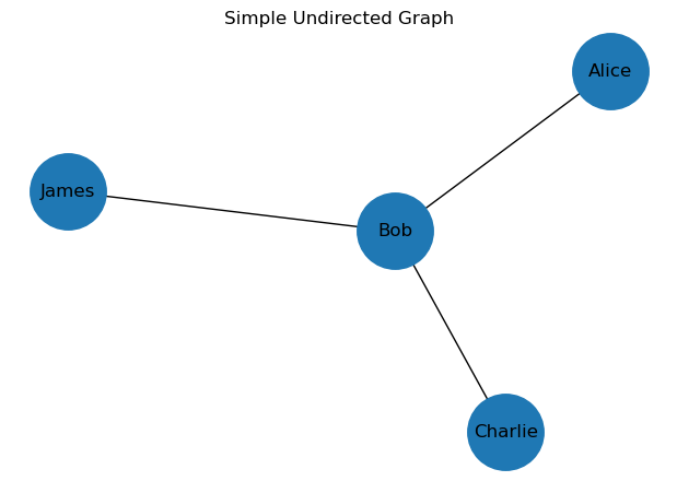
Nodes: ['Alice', 'Bob', 'Charlie', 'James'] ['Alice', 'Bob', 'Charlie', 'James']
Edges: [('Alice', 'Bob'), ('Bob', 'Charlie'), ('Bob', 'James')]
Visualizing a Graph
NetworkX integrates naturally with Matplotlib for graph visualization.
Several graph layout algorithms exist:
- spring_layout
- circular_layout
- shell_layout
- spectral_layout
- kamada_kawai_layout
2. Adding Attributes
Nodes and edges can contain arbitrary metadata.
This is extremely important in practical graph analytics.
Code
[('Alice', {'age': 25}), ('Bob', {'age': 31, 'income': array([31000,     2])}), ('Charlie', {}), ('James', {})]
[('Alice', 'Bob', {'weight': 3.7, 'friend_score': 0.5}), ('Bob', 'Charlie', {}), ('Bob', 'James', {})]
3. Directed Graphs
Directed graphs encode asymmetric relationships.
Examples:
- Twitter follows
- Web hyperlinks
- Citation networks
- Control systems
Code
Directed Edges:
['Paper A', 'Paper B', 'Paper C']
[('Paper A', 'Paper B'), ('Paper B', 'Paper C'), ('Paper C', 'Paper A')]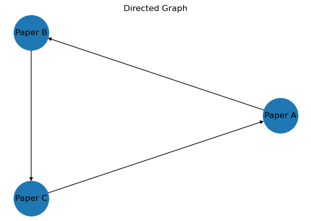
4. Weighted Graphs
Weighted graphs assign numerical values to edges.
Applications:
- Distance
- Cost
- Similarity
- Capacity
- Communication strength
Code
WG = nx.Graph()

WG.add_edge("A", "B", weight=4)
WG.add_edge("A", "C", weight=2)
WG.add_edge("B", "C", weight=1)
WG.add_edge("C", "D", weight=7)

weights = nx.get_edge_attributes(WG, "weight")

plt.figure(figsize=(6,4))

pos = nx.spring_layout(WG, seed=7)

nx.draw(
    WG,
    pos,
    with_labels=True,
    node_size=2500
)

nx.draw_networkx_edge_labels(
    WG,
    pos,
    edge_labels=weights
)

plt.title("Weighted Graph")
plt.show()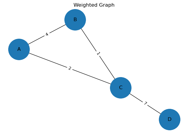
5. Graph Statistics
Graph analytics often begins with basic descriptive statistics.
Code
Number of Nodes: 4
Number of Edges: 4
Density: 0.6666666666666666
Average Clustering Coefficient: 0.5833333333333334
Degree
The degree of a node is the number of connections it has.
In directed graphs:
- in-degree
- out-degree
Code
<class 'dict'>
{'A': 2, 'B': 2, 'C': 3, 'D': 1}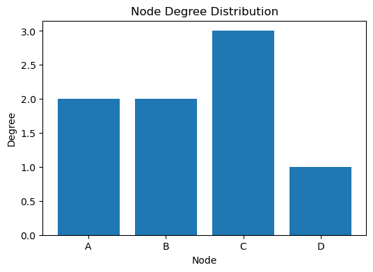
6. Shortest Paths
Shortest path algorithms are foundational in:
- GPS routing
- Robotics
- Packet routing
- Recommendation systems
7. Centrality Measures
Centrality quantifies node importance.
Important metrics include:
- Degree Centrality
- Betweenness Centrality
- Closeness Centrality
- Eigenvector Centrality
- PageRank
Code
Degree Centrality
<class 'dict'>
{'A': 0.6666666666666666, 'B': 0.6666666666666666, 'C': 1.0, 'D': 0.3333333333333333}

Betweenness Centrality
{'A': 0.0, 'B': 0.0, 'C': 0.6666666666666666, 'D': 0.0}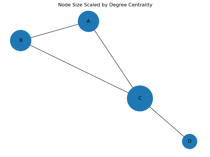
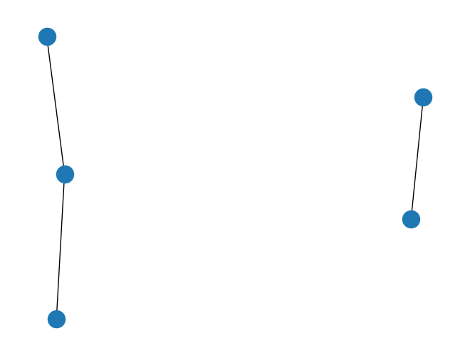
8. Connected Components
A connected component is a subset of nodes where all nodes are reachable from one another.
9. Random Graph Models
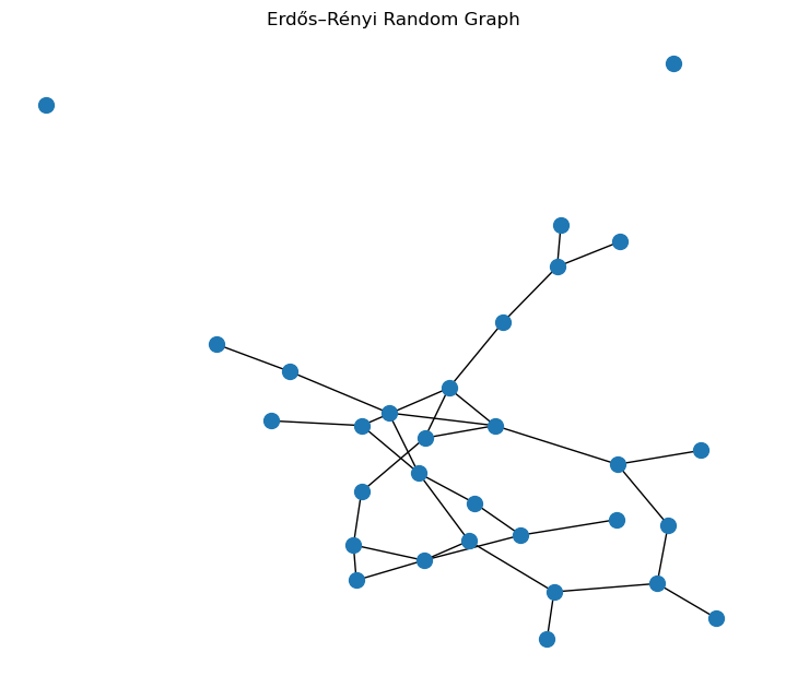
Synthetic graph models are widely used in research.
Examples: - Erdős–Rényi random graphs - Barabási–Albert scale-free networks - Watts–Strogatz small-world networks
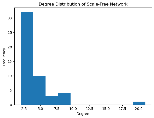
Scale-Free Networks
Many real-world networks approximately follow power-law degree distributions.
Examples: - Internet topology - Citation networks - Social media graphs
10. PageRank
PageRank is one of the most influential graph algorithms ever developed.
Originally developed by Google to rank webpages.
11. Reading and Writing Graphs
Graphs can be imported/exported in multiple formats:
- GEXF
- GraphML
- GML
- Edge lists
- JSON
12. Real-World Example: Social Network
Below is a simple synthetic social interaction graph.
Code
social = nx.Graph()

social_edges = [
    ("Alice", "Bob"),
    ("Alice", "Charlie"),
    ("Bob", "David"),
    ("Charlie", "Eve"),
    ("Eve", "Frank"),
    ("David", "Frank"),
    ("Bob", "Charlie")
]
social.add_edges_from(social_edges)

plt.figure(figsize=(8,6))

pos = nx.spring_layout(social, seed=4)

centrality = nx.degree_centrality(social)

sizes = [5000 * centrality[n] for n in social.nodes()]

nx.draw(
    social,
    pos,
    with_labels=True,
    node_size=sizes
)

plt.title("Synthetic Social Network")
plt.show()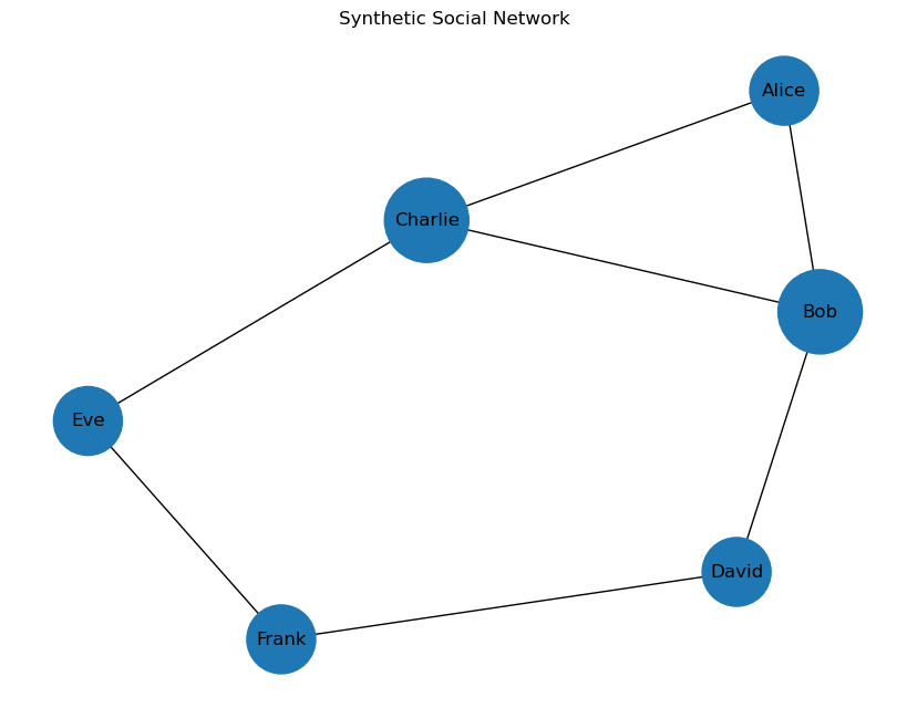
13. Adjacency Matrices
Graphs can be represented as matrices.
This is especially important in: - Spectral graph theory - Graph neural networks - Scientific computing
Code
| Alice | Bob | Charlie | David | Eve | Frank | |
|---|---|---|---|---|---|---|
| Alice | 0.0 | 1.0 | 1.0 | 0.0 | 0.0 | 0.0 |
| Bob | 1.0 | 0.0 | 1.0 | 1.0 | 0.0 | 0.0 |
| Charlie | 1.0 | 1.0 | 0.0 | 0.0 | 1.0 | 0.0 |
| David | 0.0 | 1.0 | 0.0 | 0.0 | 0.0 | 1.0 |
| Eve | 0.0 | 0.0 | 1.0 | 0.0 | 0.0 | 1.0 |
| Frank | 0.0 | 0.0 | 0.0 | 1.0 | 1.0 | 0.0 |
Summary
In this notebook you learned:
- Core graph concepts
- Creating and visualizing graphs
- Directed and weighted graphs
- Graph statistics
- Centrality measures
- Shortest paths
- Random graph models
- PageRank
- Import/export workflows
- Connections to modern graph machine learning
NetworkX remains one of the most important educational and prototyping tools for graph analytics in Python.