— because everything you learn here (windowing, chronological splitting, scaling, regularization, diagnostics) transfers unchanged to LSTMs, GRUs, and Transformers. Only the cell changes.
Roadmap
Section
Data
Task
1
One synthetic series (exponential trend + 2 sinusoids + noise)
import numpy as npimport pandas as pdimport matplotlib.pyplot as pltimport kerasfrom keras import layersfrom sklearn.metrics import mean_absolute_error, mean_squared_error, r2_scoreSEED =42keras.utils.set_random_seed(SEED) # seeds python, numpy, and tensorflow at onceplt.rcParams.update({"figure.dpi": 110, "font.size": 10, "axes.grid": True,"grid.alpha": 0.3, "axes.spines.top": False, "axes.spines.right": False,})C = {"train": "#2c7fb8", "val": "#f0a500", "test": "#d62728", "pred": "#000000"}print("Keras", keras.__version__)
Keras 2.13.1
Shared helpers
Four small functions carry the entire notebook. Read them once — they are reused verbatim in Section 2.
make_series — the data-generating process (DGP).
make_windows — turns a 1-D series into supervised (X, y) pairs.
regression_metrics — MAE / RMSE / R² / MAPE in one dict.
plot_history — training curves.
# Data-generating process: exponential trend + two sinusoids + Gaussian noise.# y(t) = level*exp(growth*t) + a1*sin(2*pi*t/p1) + a2*sin(2*pi*t/p2 + phase) + epsdef make_series(n, level, growth, a1, p1, a2, p2, phase, noise, rng): t = np.arange(n) trend = level * np.exp(growth * t) # slow multiplicative growth seasonal = (a1 * np.sin(2* np.pi * t / p1) # long oscillation+ a2 * np.sin(2* np.pi * t / p2 + phase)) # short oscillation eps = noise * rng.standard_normal(n) # irreducible noise -> sets the error floorreturn trend + seasonal + eps, trend, seasonal, eps# Slide a window of length `window` over `series`; the target is the value `horizon` steps after# the window ends. X -> (samples, window, features); y -> (samples, features)def make_windows(series, window, horizon=1): series = np.asarray(series)if series.ndim ==1: # (T,) -> (T, 1) so univariate and multivariate share code series = series[:, None] X, y = [], []for i inrange(len(series) - window - horizon +1): X.append(series[i : i + window]) # inputs: t-window ... t-1 y.append(series[i + window + horizon -1]) # target: t (one step ahead)return np.array(X), np.array(y)def regression_metrics(y_true, y_pred):return {"MAE": mean_absolute_error(y_true, y_pred),"RMSE": np.sqrt(mean_squared_error(y_true, y_pred)),"R2": r2_score(y_true, y_pred),"MAPE%": 100* np.mean(np.abs((y_true - y_pred) / y_true)), }# Loss (MSE) and MAE vs epoch, train vs validation.def plot_history(history, title="Learning curves"): h = history.history fig, ax = plt.subplots(1, 2, figsize=(10, 3.4))for a, key, name inzip(ax, ["loss", "mae"], ["Loss (MSE, scaled units)", "MAE (scaled units)"]): a.plot(h[key], color=C["train"], label="train") a.plot(h["val_"+ key], color=C["val"], label="validation") best =int(np.argmin(h["val_"+ key])) a.axvline(best, ls=":", c="grey") a.scatter([best], [h["val_"+ key][best]], c=C["val"], zorder=5) a.set(xlabel="epoch", ylabel=name, yscale="log") a.legend(frameon=False) fig.suptitle(title) fig.tight_layout() plt.show()
Section 1 — Univariate time series
1.1 Generate and inspect the data
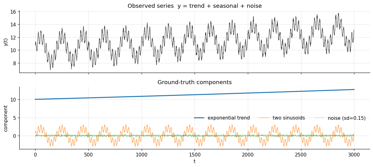
We build the series from three transparent ingredients so we always know the ground truth: a gentle exponential trend, two sinusoids of different periods, and small Gaussian noise.
The noise is the irreducible part: no model can do better than its standard deviation. That gives us a target to compare against.
N =3000WINDOW =40# how many past steps the RNN seesHORIZON =1# predict one step aheadrng = np.random.default_rng(SEED)y, trend, seasonal, eps = make_series( n=N, level=10.0, growth=8e-5, # trend: 10 -> ~12.7 over the run a1=2.0, p1=200, # slow oscillation, period 200 a2=1.0, p2=25, phase=0.8, # fast oscillation, period 25 noise=0.15, rng=rng,)t = np.arange(N)fig, ax = plt.subplots(2, 1, figsize=(11, 5), sharex=True)ax[0].plot(t, y, lw=0.8, color="#333")ax[0].set(ylabel="y(t)", title="Observed series y = trend + seasonal + noise")ax[1].plot(t, trend, label="exponential trend", lw=2)ax[1].plot(t, seasonal, label="two sinusoids", lw=0.8, alpha=0.9)ax[1].plot(t, eps, label=f"noise (sd={eps.std():.2f})", lw=0.5, alpha=0.6)ax[1].set(xlabel="t", ylabel="component", title="Ground-truth components")ax[1].legend(frameon=False, ncol=3)fig.tight_layout(); plt.show()print(f"Irreducible noise sd = {eps.std():.3f} -> the best achievable RMSE")
Irreducible noise sd = 0.151 -> the best achievable RMSE
1.2 Chronological split
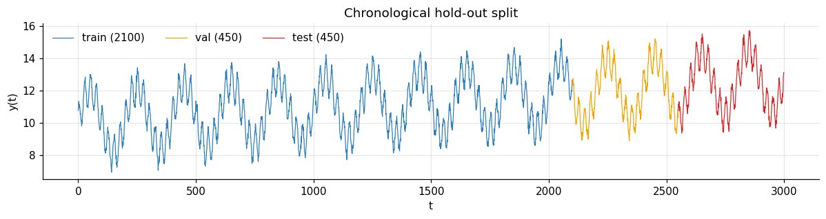
The single most important rule in time-series ML: never shuffle before splitting. A random split lets the model see the future, and your validation score becomes a lie.
We cut the series in time: the first 70 % trains, the next 15 % validates, the last 15 % tests.
Note the small overlap we allow: to build a window whose target is the first test point, the model must look at the last WINDOW points of validation. That is legitimate — those are past observations at prediction time. What matters is that no target ever appears in two splits.
n_train =int(0.70* N)n_val =int(0.15* N)# raw (unscaled) slices; val/test carry WINDOW points of history so their first target is predictabletrain_raw = y[:n_train]val_raw = y[n_train - WINDOW : n_train + n_val]test_raw = y[n_train + n_val - WINDOW :]fig, ax = plt.subplots(figsize=(11, 3))ax.plot(t[:n_train], y[:n_train], color=C["train"], lw=0.8, label=f"train ({n_train})")ax.plot(t[n_train:n_train+n_val], y[n_train:n_train+n_val], color=C["val"], lw=0.8, label=f"val ({n_val})")ax.plot(t[n_train+n_val:], y[n_train+n_val:], color=C["test"], lw=0.8, label=f"test ({N-n_train-n_val})")ax.set(xlabel="t", ylabel="y(t)", title="Chronological hold-out split")ax.legend(frameon=False, ncol=3); fig.tight_layout(); plt.show()
1.3 Scale — using training statistics only
Neural nets train best on inputs of order 1. We standardize with
The mean and standard deviation come only from the training slice. Using the full series would leak information about the future into the model — a subtle but very common bug.
mu, sd = train_raw.mean(), train_raw.std() # <- fitted on TRAIN ONLYscale =lambda a: (a - mu) / sdunscale =lambda a: a * sd + muX_tr, y_tr = make_windows(scale(train_raw), WINDOW, HORIZON)X_va, y_va = make_windows(scale(val_raw), WINDOW, HORIZON)X_te, y_te = make_windows(scale(test_raw), WINDOW, HORIZON)print(f"train mu={mu:.3f} sd={sd:.3f}")for name, X, yy in [("train", X_tr, y_tr), ("val", X_va, y_va), ("test", X_te, y_te)]:print(f"{name:>5}: X {X.shape} y {yy.shape}")
train mu=10.941  sd=1.675
train: X (2060, 40, 1)  y (2060, 1)
  val: X (450, 40, 1)  y (450, 1)
 test: X (450, 40, 1)  y (450, 1)
X has shape (samples, timesteps, features) — the shape every Keras recurrent layer expects. Here features = 1 because the series is univariate. In Section 2 only that last number changes.
1.4 Build the model
Standard practice for a first recurrent baseline:
Two stacked SimpleRNN layers. The first returns the full sequence (return_sequences=True) so the second can consume it; the second returns only the final hidden state \(h_T\) — a fixed-length summary of the window.
Dropout as the regularizer — the standard, default choice. Randomly zeroing activations during training stops the network from over-relying on any single unit. Rates of 0.1–0.3 are typical; with a small recurrent net, too much dropout simply underfits, so we start at 0.1.
Dense(1) head, linear activation — this is regression, so no squashing at the output.
MSE loss, the canonical regression loss; we also monitor MAE because it is in interpretable units.
def build_rnn(window, n_features, n_outputs, units=32, dropout=0.1): model = keras.Sequential([ keras.Input(shape=(window, n_features)), layers.SimpleRNN(units, return_sequences=True), # sequence -> sequence layers.Dropout(dropout), # regularization layers.SimpleRNN(units), # sequence -> final hidden state layers.Dropout(dropout), layers.Dense(n_outputs), # linear head for regression ]) model.compile(optimizer=keras.optimizers.Adam(1e-3), loss="mse", metrics=["mae"])return modelmodel = build_rnn(WINDOW, n_features=1, n_outputs=1)model.summary()
WARNING:absl:At this time, the v2.11+ optimizer `tf.keras.optimizers.Adam` runs slowly on M1/M2 Macs, please use the legacy Keras optimizer instead, located at `tf.keras.optimizers.legacy.Adam`.
WARNING:absl:There is a known slowdown when using v2.11+ Keras optimizers on M1/M2 Macs. Falling back to the legacy Keras optimizer, i.e., `tf.keras.optimizers.legacy.Adam`.
Two callbacks do the heavy lifting, and both are regularizers in their own right:
EarlyStopping halts training once validation loss stops improving and — crucially — restore_best_weights=True rolls the model back to its best epoch. This is early stopping, the cheapest form of regularization there is.
ReduceLROnPlateau anneals the learning rate when progress stalls, letting the optimizer settle into a sharper minimum.
callbacks = [ keras.callbacks.EarlyStopping(monitor="val_loss", patience=20, restore_best_weights=True), keras.callbacks.ReduceLROnPlateau(monitor="val_loss", factor=0.5, patience=8, min_lr=1e-5),]history = model.fit( X_tr, y_tr, validation_data=(X_va, y_va), epochs=150, batch_size=64, shuffle=True, # OK: the *windows* may be shuffled, the series was never shuffled callbacks=callbacks, verbose=0,)print(f"stopped after {len(history.history['loss'])} epochs; "f"best val_loss = {min(history.history['val_loss']):.5f}")
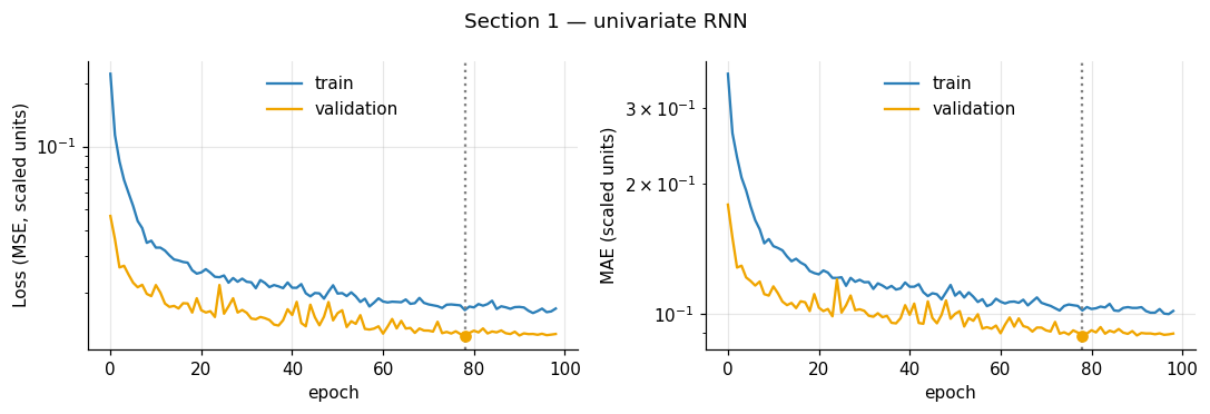
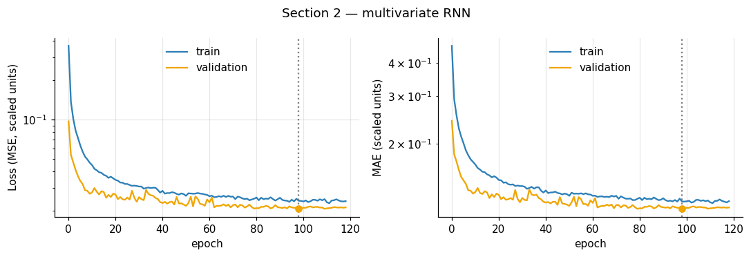
stopped after 99 epochs; best val_loss = 0.01243
1.6 Diagnose the training run
The two curves should descend together. A validation curve that turns upward while training keeps falling is the signature of overfitting — the dotted line marks the epoch EarlyStopping restored.
Predictions are made in scaled space, then mapped back to the original units with \(y = z\,\sigma_{\text{train}} + \mu_{\text{train}}\) so every metric below is in the units of the data.
We also compute a persistence baseline (\(\hat{y}_t = y_{t-1}\), “tomorrow looks like today”). Any forecasting model that cannot beat persistence has learned nothing useful.
def evaluate(model, X, y_scaled, unscale_fn): y_true = unscale_fn(y_scaled).ravel() y_pred = unscale_fn(model.predict(X, verbose=0)).ravel()return y_true, y_predrows = {}for name, X, ys in [("train", X_tr, y_tr), ("val", X_va, y_va), ("test", X_te, y_te)]: yt, yp = evaluate(model, X, ys, unscale) rows[f"RNN ({name})"] = regression_metrics(yt, yp)# persistence baseline on the test set: predict the last observed value of each windowy_true_te, y_pred_te = evaluate(model, X_te, y_te, unscale)y_naive_te = unscale(X_te[:, -1, 0])rows["Persistence (test)"] = regression_metrics(y_true_te, y_naive_te)pd.DataFrame(rows).T.round(4)
MAE
RMSE
R2
MAPE%
RNN (train)
0.1381
0.1743
0.9893
1.2948
RNN (val)
0.1481
0.1867
0.9863
1.2536
RNN (test)
0.1625
0.2085
0.9820
1.3194
Persistence (test)
0.2291
0.2837
0.9667
1.8821
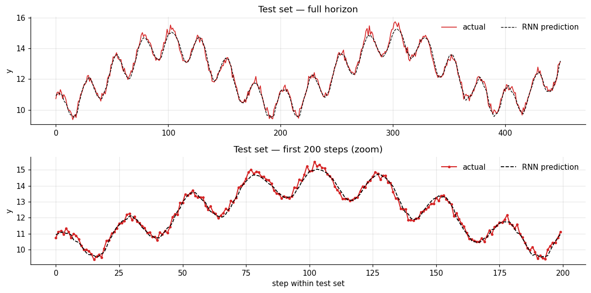
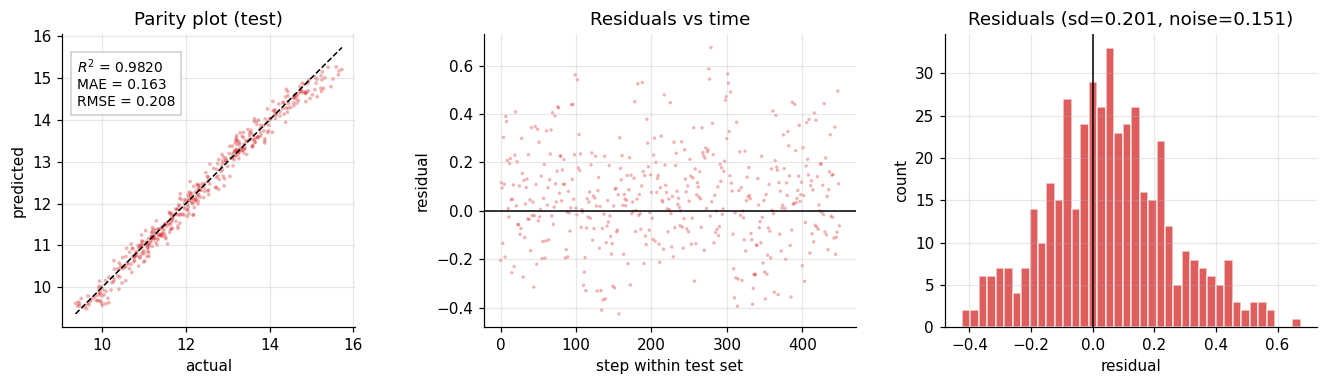
The RNN should beat persistence comfortably and land close to the noise floor (RMSE \(\approx\) 0.15) — that is the sign of a model that has learned the signal and is no longer able to do better only because the remaining error is pure randomness.
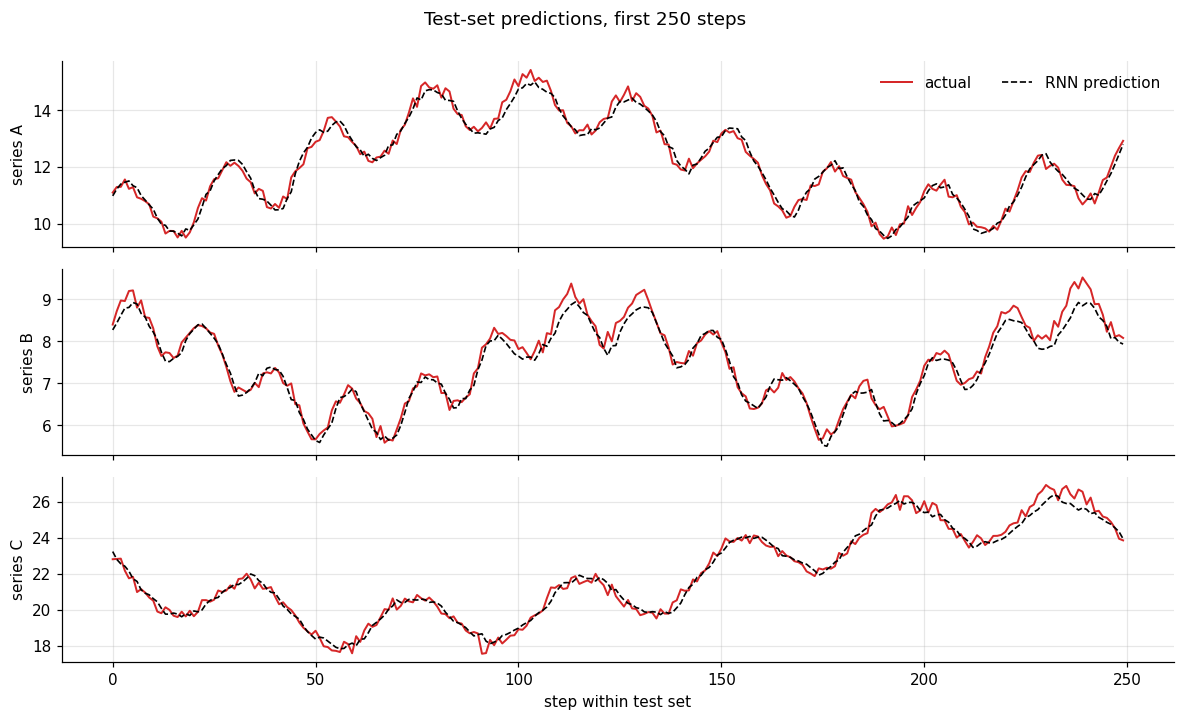
fig, ax = plt.subplots(2, 1, figsize=(11, 5.5))ax[0].plot(y_true_te, color=C["test"], lw=1.1, label="actual")ax[0].plot(y_pred_te, color=C["pred"], lw=0.9, ls="--", label="RNN prediction")ax[0].set(ylabel="y", title="Test set — full horizon"); ax[0].legend(frameon=False, ncol=2)z =slice(0, 200) # zoom in: at full width the two curves lie on top of each otherax[1].plot(y_true_te[z], color=C["test"], lw=1.4, marker="o", ms=2.5, label="actual")ax[1].plot(y_pred_te[z], color=C["pred"], lw=1.2, ls="--", label="RNN prediction")ax[1].set(xlabel="step within test set", ylabel="y", title="Test set — first 200 steps (zoom)")ax[1].legend(frameon=False, ncol=2)fig.tight_layout(); plt.show()
Parity plot and residual diagnostics
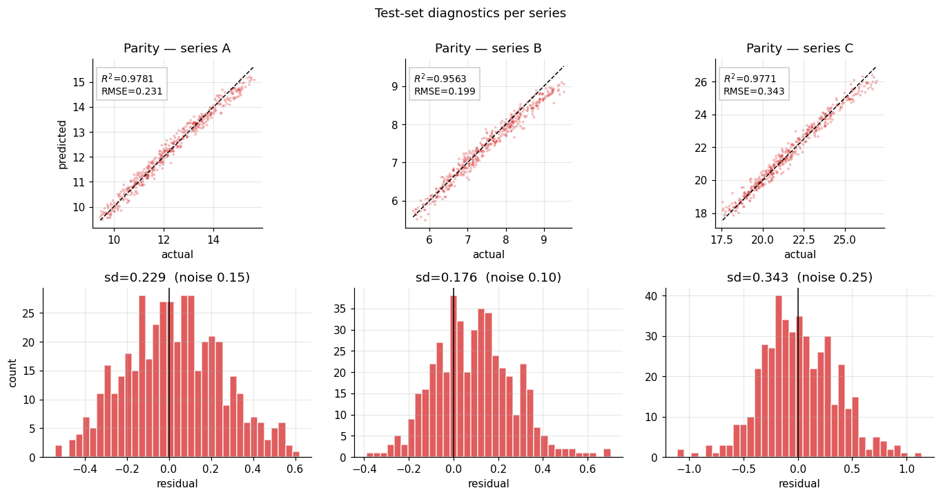
Parity plot — predicted vs actual. Perfect predictions sit on the 45° line; systematic curvature or a slope \(\neq 1\) reveals bias.
Residuals vs time — should look like structureless noise. Any leftover pattern (drift, oscillation) is signal the model failed to capture.
Residual histogram — should be centred at zero, roughly Gaussian, with a spread close to the irreducible noise level.
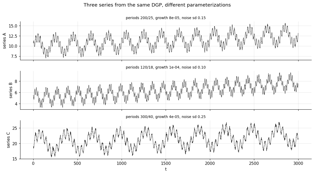
Same DGP, three different parameterizations: different growth rates, amplitudes, periods, phases and noise levels. The three series are stacked into a matrix of shape (T, 3).
What changes: the input window becomes (WINDOW, 3) and the output head becomes Dense(3). The RNN now consumes all three channels at every timestep and predicts the next value of all three at once, so it can exploit any shared structure across them.
What does not change: every other line of the workflow.
PARAMS = [dict(name="A", level=10.0, growth=8.0e-5, a1=2.0, p1=200, a2=1.0, p2=25, phase=0.8, noise=0.15),dict(name="B", level=5.0, growth=1.5e-4, a1=1.2, p1=120, a2=0.6, p2=18, phase=2.1, noise=0.10),dict(name="C", level=20.0, growth=4.0e-5, a1=3.0, p1=300, a2=1.5, p2=40, phase=4.0, noise=0.25),]NAMES = [p["name"] for p in PARAMS]K =len(PARAMS)rng = np.random.default_rng(SEED +1)series, noises = [], []for p in PARAMS: q = {k: v for k, v in p.items() if k !="name"} s, _, _, e = make_series(n=N, rng=rng, **q) series.append(s); noises.append(e.std())Y = np.column_stack(series) # (T, 3)fig, ax = plt.subplots(K, 1, figsize=(11, 6), sharex=True)for k inrange(K): ax[k].plot(t, Y[:, k], lw=0.7, color="#333") ax[k].set(ylabel=f"series {NAMES[k]}") ax[k].set_title(f"periods {PARAMS[k]['p1']}/{PARAMS[k]['p2']}, "f"growth {PARAMS[k]['growth']:.0e}, noise sd {noises[k]:.2f}", fontsize=9)ax[-1].set_xlabel("t")fig.suptitle("Three series from the same DGP, different parameterizations", y=1.0)fig.tight_layout(); plt.show()
2.1 Split, scale, window
Identical to Section 1, with two details generalized:
the split is applied to rows of the matrix, so all three channels are cut at the same instants;
scaling is per column — each series has its own \(\mu, \sigma\) from the training rows, because their levels and spreads differ by design.
Same architecture, wider (64 units) because there are now three interacting channels to model, and a three-unit output head. Same regularization: dropout + early stopping + LR annealing. Note that the extra width is doing real work here — with only 32 units the shared hidden state cannot represent three different oscillation periods at once and the model fails to beat persistence.
WARNING:absl:At this time, the v2.11+ optimizer `tf.keras.optimizers.Adam` runs slowly on M1/M2 Macs, please use the legacy Keras optimizer instead, located at `tf.keras.optimizers.legacy.Adam`.
WARNING:absl:There is a known slowdown when using v2.11+ Keras optimizers on M1/M2 Macs. Falling back to the legacy Keras optimizer, i.e., `tf.keras.optimizers.legacy.Adam`.
The loss is the average MSE across the three channels, so we now report metrics per series — an aggregate number could hide one badly-fit channel behind two good ones. Check that the RNN beats persistence on every series, not just on average.
Windowing turns forecasting into supervised regression.(samples, timesteps, features) is the only tensor shape you need to remember; univariate and multivariate differ only in features.
Split by time, never at random, and fit the scaler on the training slice alone. These two rules prevent the overwhelming majority of “my model was great in validation and useless in production”.
Regularize with dropout + early stopping. The learning curves tell you immediately whether you have the capacity/regularization balance right.
Always compare against a naive baseline. Persistence is free and surprisingly hard to beat.
Judge the model against the noise floor. Residuals whose standard deviation approaches the irreducible noise mean the model has extracted essentially all the available signal — pushing further only fits noise.
Natural extensions
Swap SimpleRNN for LSTM or GRU — a one-line change — and compare. Vanilla RNNs struggle to propagate gradients across long windows; that is exactly what gated cells were invented to fix.
Forecast further ahead (HORIZON > 1), or emit a whole trajectory (Dense(H)), or feed predictions back in autoregressively and watch the errors compound.
Our exponential trend is mild, so the test values stay inside the training range. Push the growth rate up and the model will systematically under-predict: an RNN interpolates, it does not extrapolate a trend it has never seen. The standard remedies are differencing the series or normalizing each window by its own last value.
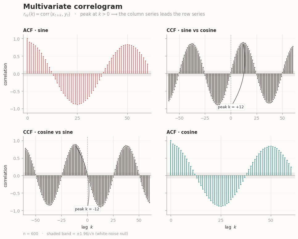
"""Multivariate correlogram ("cross-correlation matrix plot").Diagonal : autocorrelation function (ACF) of each seriesOff-diagonal: cross-correlation function (CCF) over +/- lagsSign convention (Box-Jenkins): r_xy(k) = corr(x[t+k], y[t])A peak at POSITIVE k means y LEADS x by k steps."""import numpy as npimport matplotlib.pyplot as pltfrom matplotlib.ticker import MultipleLocator# ----------------------------------------------------------------------# Correlation machinery# ----------------------------------------------------------------------def ccf(x, y, maxlag):"""Cross-correlation r_xy(k) = corr(x[t+k], y[t]) for k in [-maxlag, maxlag].""" x = np.asarray(x, float) y = np.asarray(y, float) n =len(x) xc = x - x.mean() yc = y - y.mean() denom = n * x.std() * y.std() lags = np.arange(-maxlag, maxlag +1) r = np.empty_like(lags, dtype=float)for i, k inenumerate(lags):if k >=0: r[i] = np.dot(xc[k:], yc[: n - k]) / denomelse: r[i] = np.dot(xc[: n + k], yc[-k:]) / denomreturn lags, rdef acf(x, maxlag):"""One-sided autocorrelation, lags 0..maxlag.""" lags, r = ccf(x, x, maxlag)return lags[maxlag:], r[maxlag:]# ----------------------------------------------------------------------# Sample data: cosine leads sine by a quarter period# ----------------------------------------------------------------------rng = np.random.default_rng(7)N =600# samplesPERIOD =50# samples per cycleMAXLAG =60# lags to displayNOISE =0.25t = np.arange(N)s1 = np.sin(2* np.pi * t / PERIOD) + NOISE * rng.standard_normal(N)s2 = np.cos(2* np.pi * t / PERIOD) + NOISE * rng.standard_normal(N)series = {"sine": s1, "cosine": s2}names =list(series)k =len(names)# ----------------------------------------------------------------------# Style# ----------------------------------------------------------------------INK ="#2B2B2B"MUTED ="#9A9A94"GRID ="#E6E4DF"BAND ="#B9B5AC"PAPER ="#FDFCF9"COLORS = {"sine": "#C1666B", "cosine": "#3C8D8A"} # rose / tealCROSS ="#6B6560"# neutral for off-diagonalplt.rcParams.update({"font.family": "DejaVu Sans","font.size": 9,"axes.edgecolor": MUTED,"axes.linewidth": 0.8,"xtick.color": MUTED,"ytick.color": MUTED,"xtick.direction": "out","ytick.direction": "out",})conf =1.96/ np.sqrt(N) # white-noise band -- see caveat in the write-updef stems(ax, lags, r, color): ax.vlines(lags, 0, r, color=color, lw=1.5, alpha=0.85, zorder=3) ax.plot(lags, r, "o", ms=3.0, color=color, mec=PAPER, mew=0.6, zorder=4)# ----------------------------------------------------------------------# Figure# ----------------------------------------------------------------------fig, axes = plt.subplots( k, k, figsize=(9.2, 7.4), sharey=True, gridspec_kw=dict(hspace=0.30, wspace=0.12, left=0.10, right=0.97, top=0.83, bottom=0.11),)fig.patch.set_facecolor(PAPER)for i, row inenumerate(names): # row -> x (the "t+k" series)for j, col inenumerate(names): # col -> y (the reference series) ax = axes[i, j] ax.set_facecolor(PAPER)# confidence band + zero line ax.axhspan(-conf, conf, color=BAND, alpha=0.22, lw=0, zorder=0) ax.axhline(0, color=MUTED, lw=0.8, zorder=1)if i == j: lags, r = acf(series[row], MAXLAG) stems(ax, lags, r, COLORS[row]) ax.set_title(f"ACF · {row}", fontsize=9.5, color=INK, pad=6, loc="left", fontweight="bold") ax.set_xlim(-2, MAXLAG +2)else: lags, r = ccf(series[row], series[col], MAXLAG) stems(ax, lags, r, CROSS) ax.axvline(0, color=MUTED, lw=0.8, ls=(0, (3, 3)), zorder=1) ax.set_title(f"CCF · {row} vs {col}", fontsize=9.5, color=INK, pad=6, loc="left", fontweight="bold") ax.set_xlim(-MAXLAG -2, MAXLAG +2)# Annotate the dominant peak -> this is the lead/lag you care about.# NB: a periodic CCF has equally-good peaks every PERIOD steps, so# take the strongest POSITIVE correlation within one half-period. win = np.abs(lags) <= PERIOD //2 idx = np.flatnonzero(win)[np.argmax(r[win])] pk = lags[idx] ax.annotate(f"peak k = {pk:+d}", xy=(pk, r[idx]), xytext=(0.5, 0.06), textcoords="axes fraction", fontsize=8, color=INK, ha="center", arrowprops=dict(arrowstyle="-", lw=0.8, color=INK, shrinkA=0, shrinkB=3, connectionstyle="arc3,rad=0.2"), bbox=dict(boxstyle="round,pad=0.3", fc="white", ec=GRID, lw=0.7), ) ax.set_ylim(-1.12, 1.12) ax.grid(axis="y", color=GRID, lw=0.7, zorder=0) ax.xaxis.set_major_locator(MultipleLocator(25)) ax.yaxis.set_major_locator(MultipleLocator(0.5))for side in ("top", "right"): ax.spines[side].set_visible(False) ax.spines["left"].set_color(MUTED) ax.spines["bottom"].set_color(MUTED)if i == k -1: ax.set_xlabel("lag $k$", color=INK, fontsize=9)if j ==0: ax.set_ylabel("correlation", color=INK, fontsize=9)fig.suptitle("Multivariate correlogram", x=0.10, y=0.955, ha="left", fontsize=15, color=INK, fontweight="bold")fig.text(0.10, 0.905,r"$r_{xy}(k)=\mathrm{corr}\,(x_{t+k},\,y_t)$ · ""peak at $k>0$ ⟹ the column series leads the row series", ha="left", fontsize=9.5, color=MUTED)fig.text(0.10, 0.030,f"n = {N} · shaded band = ±1.96/√n (white-noise null)", ha="left", fontsize=8, color=MUTED)fig.savefig("correlogram.png", dpi=200, facecolor=PAPER)plt.show()# Sanity check: the recovered lead/lag should be the quarter period.lags, r = ccf(s1, s2, MAXLAG)win = np.abs(lags) <= PERIOD //2print(f"recovered peak lag : {lags[np.flatnonzero(win)[np.argmax(r[win])]]:+d}")print(f"quarter period : {PERIOD /4:+.1f}")
recovered peak lag : +12
quarter period     : +12.5
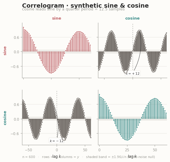
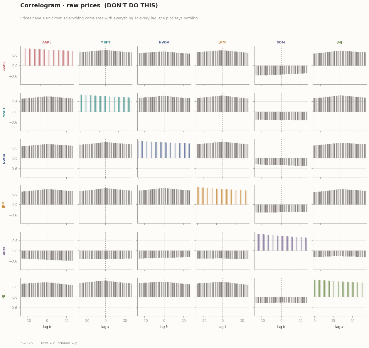
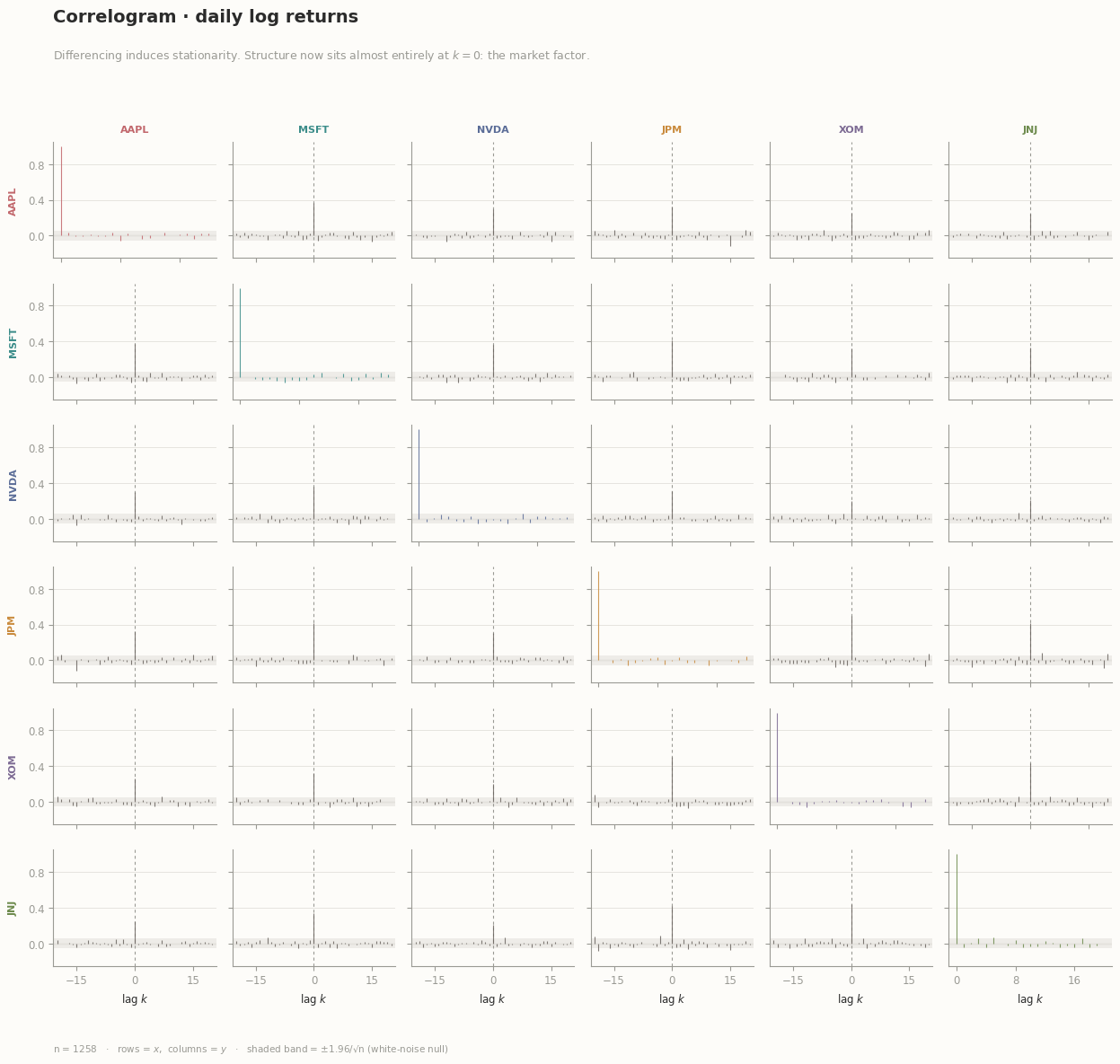
"""Multivariate correlogram: a pair-plot for time series. diagonal -> autocorrelation (ACF) of each series off-diagonal -> cross-correlation (CCF) over +/- lagsSign convention (Box-Jenkins): r_xy(k) = corr( x[t+k], y[t] )so in panel (row = x, col = y), a peak at POSITIVE k means the COLUMNseries LEADS the ROW series by k steps.Since r_xy(k) = r_yx(-k), the upper and lower triangles are mirror images.That redundancy is deliberate: each panel is independently readable.(R's acf() halves it, showing +lags above the diagonal and -lags below.)Self-contained: numpy + pandas + matplotlib only."""import numpy as npimport pandas as pdimport matplotlib.pyplot as pltfrom matplotlib.ticker import MaxNLocatorMAX_SERIES =6# ==========================================================================# Correlation machinery# ==========================================================================def ccf(x, y, maxlag):"""Cross-correlation r_xy(k) = corr(x[t+k], y[t]) for k in [-maxlag, maxlag].""" x = np.asarray(x, dtype=float) y = np.asarray(y, dtype=float)if x.shape != y.shape:raiseValueError("x and y must have the same length") ok = np.isfinite(x) & np.isfinite(y) x, y = x[ok], y[ok] n = x.sizeif n <= maxlag:raiseValueError(f"need more than maxlag={maxlag} valid points, got {n}") xc, yc = x - x.mean(), y - y.mean() denom = n * x.std() * y.std()if denom ==0:raiseValueError("a series is constant; correlation undefined") lags = np.arange(-maxlag, maxlag +1) r = np.empty(lags.size, dtype=float)for i, k inenumerate(lags):if k >=0: r[i] = np.dot(xc[k:], yc[: n - k]) / denomelse: r[i] = np.dot(xc[: n + k], yc[-k:]) / denomreturn lags, rdef acf(x, maxlag):"""One-sided autocorrelation, lags 0..maxlag.""" lags, r = ccf(x, x, maxlag)return lags[maxlag:], r[maxlag:]# ==========================================================================# The plot# ==========================================================================INK, MUTED, GRID, BAND, PAPER ="#2B2B2B", "#9A9A94", "#E6E4DF", "#B9B5AC", "#FDFCF9"CROSS ="#6B6560"PALETTE = ["#C1666B", "#3C8D8A", "#5A6C97", "#C98A3C", "#7C6A93", "#6E8B4E"]def correlogram_matrix( series, names=None, maxlag=40, conf=True, annotate_peak=None, # None -> auto (on for <= 3 series) peak_window=None, # restrict peak search to |k| <= this ylim=None, title="Multivariate correlogram", subtitle=None, figsize=None,):"""ACF/CCF matrix for up to six time series. series : list of 1-D arrays, or a DataFrame (columns = series) names : list of str; taken from DataFrame columns if omitted conf : draw the +/- 1.96/sqrt(n) white-noise band (valid only under a white-noise null -- see the prices-vs-returns demo below) peak_window : for periodic data, whose CCF has equally-good peaks every period, search the peak only within |k| <= peak_window Returns (fig, axes). """# ---- unpack -----------------------------------------------------------ifhasattr(series, "columns"): # DataFrameif names isNone: names = [str(c) for c in series.columns] series = [series[c].to_numpy(dtype=float) for c in series.columns]else: series = [np.asarray(s, dtype=float).ravel() for s in series]if names isNone: names = [f"series {i+1}"for i inrange(len(series))] k =len(series)ifnot1<= k <= MAX_SERIES:raiseValueError(f"supply between 1 and {MAX_SERIES} series, got {k}")iflen(names) != k:raiseValueError("len(names) must match len(series)")iflen({s.size for s in series}) !=1:raiseValueError("all series must be the same length") n =min(np.isfinite(s).sum() for s in series)if annotate_peak isNone: annotate_peak = k <=3# ---- adaptive density ------------------------------------------------- dense = k >=4 lw =0.8if dense else1.5 ms =0.0if dense else3.0# drop markers once panels shrink lab_fs =8if dense else9.5if figsize isNone: figsize = (2.05* k +1.4, 1.75* k +1.9) band =1.96/ np.sqrt(n) plt.rcParams.update({"font.family": "DejaVu Sans", "font.size": 8.5,"axes.edgecolor": MUTED, "axes.linewidth": 0.8,"xtick.color": MUTED, "ytick.color": MUTED, }) fig, axes = plt.subplots( k, k, figsize=figsize, squeeze=False, sharey=True, gridspec_kw=dict(hspace=0.22, wspace=0.10, left=0.115, right=0.975, top=0.845, bottom=0.105), ) fig.patch.set_facecolor(PAPER) lo, hi =0.0, 0.0for i inrange(k): # row -> x (the "t+k" series)for j inrange(k): # col -> y (the reference series) ax = axes[i, j] ax.set_facecolor(PAPER)if conf: ax.axhspan(-band, band, color=BAND, alpha=0.22, lw=0, zorder=0) ax.axhline(0, color=MUTED, lw=0.8, zorder=1)if i == j: lags, r = acf(series[i], maxlag) color = PALETTE[i %len(PALETTE)] ax.set_xlim(-1, maxlag +1)else: lags, r = ccf(series[i], series[j], maxlag) color = CROSS ax.axvline(0, color=MUTED, lw=0.8, ls=(0, (3, 3)), zorder=1) ax.set_xlim(-maxlag -1, maxlag +1) ax.vlines(lags, 0, r, color=color, lw=lw, alpha=0.85, zorder=3)if ms: ax.plot(lags, r, "o", ms=ms, color=color, mec=PAPER, mew=0.6, zorder=4) lo, hi =min(lo, r.min()), max(hi, r.max())if i != j and annotate_peak: sel = (np.abs(lags) <= peak_window) if peak_window \else np.ones_like(lags, dtype=bool) idx = np.flatnonzero(sel)[np.argmax(r[sel])] ax.annotate(f"$k={lags[idx]:+d}$", xy=(lags[idx], r[idx]), xytext=(0.5, 0.06), textcoords="axes fraction", fontsize=7.5, color=INK, ha="center", arrowprops=dict(arrowstyle="-", lw=0.7, color=INK, shrinkA=0, shrinkB=3, connectionstyle="arc3,rad=0.2"), bbox=dict(boxstyle="round,pad=0.25", fc="white", ec=GRID, lw=0.6), ) ax.grid(axis="y", color=GRID, lw=0.7, zorder=0) ax.xaxis.set_major_locator(MaxNLocator(3, integer=True)) ax.yaxis.set_major_locator(MaxNLocator(4))for side in ("top", "right"): ax.spines[side].set_visible(False)# pair-plot margin labels: names on the outside, not on each panelif j ==0: ax.set_ylabel(names[i], color=PALETTE[i %len(PALETTE)], fontsize=lab_fs, fontweight="bold", labelpad=8)if i ==0: ax.set_title(names[j], color=PALETTE[j %len(PALETTE)], fontsize=lab_fs, fontweight="bold", pad=8)if i == k -1: ax.set_xlabel("lag $k$", color=INK, fontsize=8.5)else: ax.tick_params(labelbottom=False) pad =0.10*max(hi - lo, 0.2)for ax in axes.ravel(): ax.set_ylim((lo - pad, hi + pad) if ylim isNoneelse ylim)if subtitle isNone: subtitle = (r"$r_{xy}(k)=\mathrm{corr}(x_{t+k},\,y_t)$ · "r"peak at $k>0$ ⟹ column leads row") fig.suptitle(title, x=0.115, y=0.965, ha="left", fontsize=14, color=INK, fontweight="bold") fig.text(0.115, 0.920, subtitle, ha="left", fontsize=9, color=MUTED) foot =f"n = {n} · rows = $x$, columns = $y$"if conf: foot +=" · shaded band = ±1.96/√n (white-noise null)" fig.text(0.115, 0.028, foot, ha="left", fontsize=7.5, color=MUTED)return fig, axes# ==========================================================================# Data# ==========================================================================TICKERS = ["AAPL", "MSFT", "NVDA", "JPM", "XOM", "JNJ"]START, END ="2013-02-08", "2018-02-07"def load_prices(tickers=TICKERS, start=START, end=END):"""Daily closes as a DataFrame. Tries yfinance, falls back to a CSV."""try:import yfinance as yf df = yf.download(tickers, start=start, end=end, auto_adjust=True, progress=False)["Close"]ifnot df.empty:return df[tickers].dropna()exceptExceptionas e:print(f"[yfinance unavailable: {e}]")print("[falling back to S&P-500 daily CSV on GitHub]") url = ("https://raw.githubusercontent.com/plotly/datasets/""master/all_stocks_5yr.csv") raw = pd.read_csv(url, parse_dates=["date"])return (raw[raw["Name"].isin(tickers)] .pivot(index="date", columns="Name", values="close") .loc[start:end, tickers] .dropna())# ==========================================================================# Demo# ==========================================================================if__name__=="__main__":# --- 1. sanity check: cosine leads sine by a quarter period ------------ rng = np.random.default_rng(7) N, PERIOD =600, 50 t = np.arange(N) demo = pd.DataFrame({"sine": np.sin(2* np.pi * t / PERIOD) +0.25* rng.standard_normal(N),"cosine": np.cos(2* np.pi * t / PERIOD) +0.25* rng.standard_normal(N), }) fig, _ = correlogram_matrix( demo, maxlag=60, peak_window=PERIOD //2, title="Correlogram · synthetic sine & cosine", subtitle=f"cosine leads sine by a quarter period = {PERIOD/4:.1f} samples", ) fig.savefig("corr_sine.png", dpi=190, facecolor=fig.get_facecolor())print(f"sine/cosine: expect a peak near k = +{PERIOD/4:.1f}")# --- 2. raw prices: the WRONG way (non-stationary) --------------------- px = load_prices()print(f"\nloaded {px.shape[0]} days x {px.shape[1]} tickers "f"({px.index.min().date()} to {px.index.max().date()})") fig, _ = correlogram_matrix( px, maxlag=40, conf=False, ylim=(-1.1, 1.1), title="Correlogram · raw prices (DON'T DO THIS)", subtitle="Prices have a unit root. Everything correlates with ""everything at every lag; the plot says nothing.", ) fig.savefig("corr_prices.png", dpi=190, facecolor=fig.get_facecolor())# --- 3. log returns: the right way ------------------------------------ ret = np.log(px).diff().dropna() fig, _ = correlogram_matrix( ret, maxlag=20, ylim=(-0.25, 1.05), title="Correlogram · daily log returns", subtitle="Differencing induces stationarity. Structure now sits almost ""entirely at $k=0$: the market factor.", ) fig.savefig("corr_returns.png", dpi=190, facecolor=fig.get_facecolor())print("\nlag-0 cross-correlation of returns:")print(ret.corr().round(2).to_string()) worst =max( np.abs(ccf(ret[a], ret[b], 20)[1][ccf(ret[a], ret[b], 20)[0] !=0]).max()for a in ret.columns for b in ret.columns if a != b )print(f"\nmax |CCF| at any nonzero lag, over all pairs: {worst:.3f}")print(f"white-noise band (±1.96/√n): "f"{1.96/np.sqrt(len(ret)):.3f}") plt.show()
sine/cosine: expect a peak near k = +12.5
[yfinance unavailable: No module named 'yfinance']
[falling back to S&P-500 daily CSV on GitHub]

loaded 1259 days x 6 tickers (2013-02-08 to 2018-02-07)

lag-0 cross-correlation of returns:
Name  AAPL  MSFT  NVDA   JPM   XOM   JNJ
Name
AAPL  1.00  0.37  0.30  0.33  0.26  0.24
MSFT  0.37  1.00  0.36  0.41  0.33  0.34
NVDA  0.30  0.36  1.00  0.31  0.20  0.20
JPM   0.33  0.41  0.31  1.00  0.50  0.42
XOM   0.26  0.33  0.20  0.50  1.00  0.44
JNJ   0.24  0.34  0.20  0.42  0.44  1.00

max |CCF| at any nonzero lag, over all pairs: 0.115
white-noise band (±1.96/√n):                  0.055