LSTM Time-Series Forecasting: The Canonical Workflow
Goal: walk through the standard, end-to-end recipe for training an LSTM to forecast a bivariate time series (two channels that influence each other), with the best-practice guardrails that keep you honest: chronological splits, leakage-free scaling, a naive baseline, regularization, early stopping, and a small hyperparameter search.
The code is deliberately plain. Every cell should be readable in one pass. The point is the workflow, not clever engineering.
The workflow
Step
What
Why it matters
1
Generate / load the data
Know your signal before you model it
2
Chronological split
Shuffling a time series leaks the future
3
Scale (fit on train only)
Scaler statistics are learned parameters
4
Window into (X, y) pairs
Turns forecasting into supervised learning
5
Naive baseline
If you can’t beat it, you have no model
6
Build the LSTM
Architecture + regularization
7
Train with early stopping
Let validation loss decide when to stop
8
Small hyperparameter search
Select on validation, never on test
9
Evaluate once on test
The only unbiased number you get
10
Recursive multi-step forecast
Where errors compound
import numpy as npimport matplotlib.pyplot as pltimport tensorflow as tffrom tensorflow import kerasfrom tensorflow.keras import layersSEED =42np.random.seed(SEED)tf.random.set_seed(SEED)plt.rcParams["figure.figsize"] = (11, 4)plt.rcParams["axes.grid"] =Trueplt.rcParams["grid.alpha"] =0.3print("TensorFlow", tf.__version__)
TensorFlow 2.13.0
Step 1: Generate the data
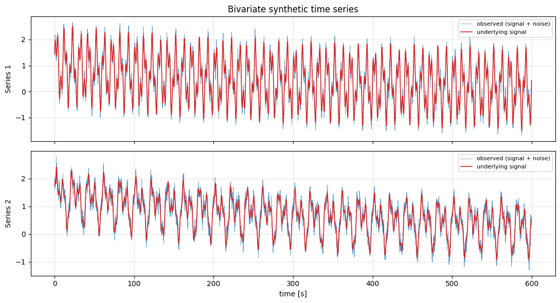
A simple generating process for each channel:
\[x(t) = \underbrace{e^{-t/\tau}}_{\text{envelope}} \cdot \underbrace{\sum_k A_k \sin(2\pi f_k t + \phi_k)}_{\text{a few sinusoids}} + \underbrace{\varepsilon(t)}_{\text{wide noise}}\]
Two things make this a good teaching signal:
The exponential envelope makes it non-stationary. The amplitude at the end of the record is not the amplitude at the beginning, so the model has to track a changing scale: and our train-only scaler will see a different range than the test set does. That is exactly the situation you face in the wild.
Channel 2 depends on a lagged copy of channel 1. That coupling is the whole reason to feed the LSTM both series: there is genuine cross-channel information to exploit.
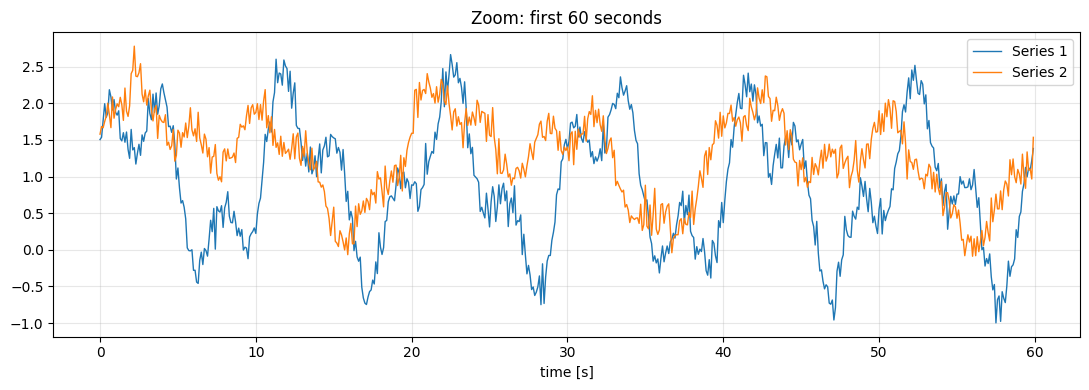
Sampling rate is 10 Hz over 600 s → 6000 samples. The fastest component (0.27 Hz) has a period of ~37 samples, the slowest (0.05 Hz) ~200 samples. Keep those numbers in mind: they set how long the lookback window needs to be.
# Zoom in so you can actually see the oscillations and how noisy the data is.zoom =slice(0, 600) # first 60 secondsplt.figure()plt.plot(t[zoom], data[zoom, 0], lw=1.0, label="Series 1")plt.plot(t[zoom], data[zoom, 1], lw=1.0, label="Series 2")plt.title("Zoom: first 60 seconds")plt.xlabel("time [s]"); plt.legend(); plt.tight_layout(); plt.show()
Step 2: Chronological train / validation / test split
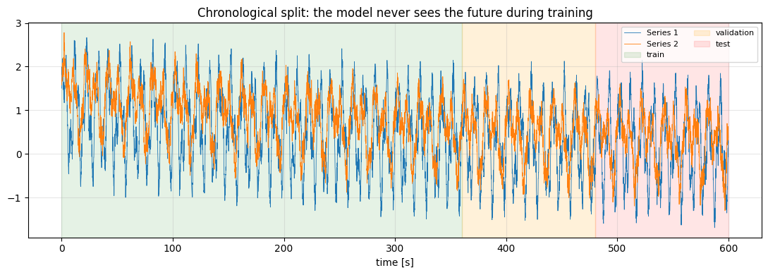
The single most common mistake in time-series ML is train_test_split(..., shuffle=True). Shuffling lets the model train on samples from after the ones it is tested on. Performance looks great and means nothing.
Split by time: earliest 60% → train, next 20% → validation, last 20% → test. The test set is a block of the future the model has never seen.
plt.figure()plt.plot(t, data[:, 0], lw=0.6, color="C0", label="Series 1")plt.plot(t, data[:, 1], lw=0.6, color="C1", label="Series 2")plt.axvspan(t[0], t[n_train -1], color="green", alpha=0.10, label="train")plt.axvspan(t[n_train], t[n_train + n_val -1], color="orange", alpha=0.15, label="validation")plt.axvspan(t[n_train + n_val], t[-1], color="red", alpha=0.10, label="test")plt.title("Chronological split: the model never sees the future during training")plt.xlabel("time [s]"); plt.legend(loc="upper right", ncol=2, fontsize=8)plt.tight_layout(); plt.show()
Step 3: Scale, fitting the scaler on the training set only
LSTMs train much better on inputs of order 1. But a scaler has learned parameters (mean and standard deviation). Compute them over the whole dataset and you have quietly told the model the mean of the test set: a subtle but real leak.
So: fit on train, transform everything.
Because of the decaying envelope, the test portion has a smaller amplitude than the training portion. After scaling with train statistics the test data will not be zero-mean, unit-variance — and that’s fine. That mismatch is the honest reflection of a non-stationary process.
mu = train_raw.mean(axis=0) # per-channel mean, from TRAIN onlysigma = train_raw.std(axis=0) # per-channel std, from TRAIN onlydef scale(a): return (a - mu) / sigmadef unscale(a): return a * sigma + mutrain = scale(train_raw)val = scale(val_raw)test = scale(test_raw)print("train mean/std:", train.mean(axis=0).round(3), train.std(axis=0).round(3))print("test mean/std:", test.mean(axis=0).round(3), test.std(axis=0).round(3)," <- not (0, 1): the series is non-stationary")
train mean/std: [ 0. -0.] [1. 1.]
test  mean/std: [-0.494 -0.905] [0.972 0.921]   <- not (0, 1): the series is non-stationary
Step 4: Window the series into supervised (X, y) pairs
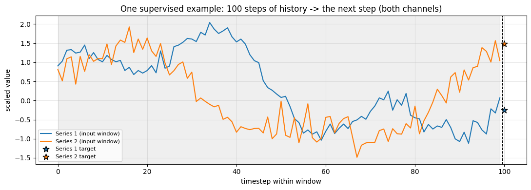
An LSTM does not consume “a time series”. It consumes a batch of fixed-length sequences. We slide a window of length LOOKBACK across the data; the window is the input X, and the value HORIZON steps after the window is the target y.
X has shape (n_windows, LOOKBACK, n_features): Keras always wants (batch, timesteps, features)
y has shape (n_windows, n_features): we predict both channels at once
LOOKBACK = 100 samples = 10 seconds, which spans a full cycle of the dominant 0.10 Hz component. Choosing the lookback shorter than the dominant period is a classic self-inflicted wound: the model literally cannot see the pattern you are asking it to learn.
Windowing each split separately is deliberate: it prevents a window from straddling the train/validation boundary.
LOOKBACK =100# timesteps of history fed to the LSTM (10 s)HORIZON =1# predict 1 step aheaddef make_windows(series, lookback=LOOKBACK, horizon=HORIZON):"""series: (timesteps, features) -> X: (windows, lookback, features), y: (windows, features)""" X, y = [], []for i inrange(len(series) - lookback - horizon +1): X.append(series[i : i + lookback]) # the past y.append(series[i + lookback + horizon -1]) # the next valuereturn np.array(X), np.array(y)X_train, y_train = make_windows(train)X_val, y_val = make_windows(val)X_test, y_test = make_windows(test)print("X_train:", X_train.shape, " y_train:", y_train.shape)print("X_val: ", X_val.shape, " y_val: ", y_val.shape)print("X_test: ", X_test.shape, " y_test: ", y_test.shape)
# What does one training example actually look like?i =300plt.figure()w = np.arange(LOOKBACK)plt.plot(w, X_train[i, :, 0], color="C0", label="Series 1 (input window)")plt.plot(w, X_train[i, :, 1], color="C1", label="Series 2 (input window)")plt.scatter([LOOKBACK], [y_train[i, 0]], color="C0", s=90, marker="*", edgecolor="k", zorder=5, label="Series 1 target")plt.scatter([LOOKBACK], [y_train[i, 1]], color="C1", s=90, marker="*", edgecolor="k", zorder=5, label="Series 2 target")plt.axvspan(0, LOOKBACK -1, color="gray", alpha=0.12)plt.axvline(LOOKBACK -0.5, color="k", ls="--", lw=1)plt.title(f"One supervised example: {LOOKBACK} steps of history -> the next step (both channels)")plt.xlabel("timestep within window"); plt.ylabel("scaled value")plt.legend(fontsize=8); plt.tight_layout(); plt.show()
Step 5: The naive baseline
Before touching a neural network, answer: what does “doing nothing” score?
The persistence (random-walk) baseline predicts that the next value equals the last observed value. For smooth, densely-sampled signals this is a surprisingly strong competitor. Many published LSTM results quietly fail to beat it.
We report RMSE and MAE in the original units, not scaled units: scaled RMSE is uninterpretable.
def rmse(a, b): returnfloat(np.sqrt(np.mean((a - b) **2)))def mae(a, b): returnfloat(np.mean(np.abs(a - b)))# Persistence: predict y_hat[t+1] = x[t] (the last value in the window)baseline_pred = X_test[:, -1, :] # (windows, features), scaledy_test_true = unscale(y_test) # back to original unitsbaseline_unscaled = unscale(baseline_pred)print(f"BASELINE (persistence) RMSE = {rmse(y_test_true, baseline_unscaled):.4f}"f" MAE = {mae(y_test_true, baseline_unscaled):.4f}")print("This is the number the LSTM has to beat.")
BASELINE (persistence)   RMSE = 0.2243   MAE = 0.1777
This is the number the LSTM has to beat.
Step 6: Build the LSTM
A small, standard architecture:
Input (LOOKBACK, 2)
  -> LSTM(units)          returns only the final hidden state
  -> Dropout(p)           regularization
  -> Dense(2)             one output per channel, linear activation
Regularization choices, and why:
Dropout after the LSTM randomly zeroes activations during training, so the Dense layer cannot depend on any single unit.
recurrent_dropout is available but slows training a lot (it disables the fast cuDNN kernel). We use the cheaper post-LSTM dropout instead.
Weight decay (L2) on the recurrent kernel keeps the weights small.
The strongest regularizer here is early stopping (next step): it caps effective model capacity by simply not training past the point where validation loss turns around.
Loss is MSE (we are doing regression); we also track MAE, which is less dominated by outliers.
1 recurrent layer model
def build_model( units=64, dropout=0.2, recurrent_dropout=0.0, # >0 disables the cuDNN fast path (see note) lr=1e-3, lookback=LOOKBACK, n_features=2, ):"""Standard single-layer LSTM regressor for multivariate one-step forecasting.""" model = keras.Sequential([ keras.Input(shape=(lookback, n_features)), layers.LSTM(units, dropout=dropout, # on the input transform recurrent_dropout=recurrent_dropout), # on the hidden-state transform layers.Dropout(dropout), # on the final representation layers.Dense(n_features), # linear head: one value per channel ]) model.compile(optimizer=keras.optimizers.Adam(learning_rate=lr), loss="mse", metrics=["mae"])return modelbuild_model().summary()
WARNING:absl:At this time, the v2.11+ optimizer `tf.keras.optimizers.Adam` runs slowly on M1/M2 Macs, please use the legacy Keras optimizer instead, located at `tf.keras.optimizers.legacy.Adam`.
WARNING:absl:There is a known slowdown when using v2.11+ Keras optimizers on M1/M2 Macs. Falling back to the legacy Keras optimizer, i.e., `tf.keras.optimizers.legacy.Adam`.
# def build_model(# units=64,# dropout=0.2,# recurrent_dropout=0.0,# lr=1e-3,# lookback=LOOKBACK,# n_features=2,# ):# """Stacked (2-layer) LSTM regressor for multivariate one-step forecasting."""# model = keras.Sequential([# keras.Input(shape=(lookback, n_features)),# layers.LSTM(units,# dropout=dropout,# recurrent_dropout=recurrent_dropout,# return_sequences=True), # pass the full sequence up# layers.LSTM(units,# dropout=dropout,# recurrent_dropout=recurrent_dropout), # collapses to a vector# layers.Dropout(dropout),# layers.Dense(n_features),# ])# model.compile(optimizer=keras.optimizers.Adam(learning_rate=lr),# loss="mse",# metrics=["mae"])# return model# build_model().summary()
N recurrent layer model
# def build_model(# units=64,# dropout=0.2,# recurrent_dropout=0.0, # >0 disables the cuDNN fast path (see note)# n_layers=1, # 1 = textbook baseline; 2 = stacked# lr=1e-3,# lookback=LOOKBACK,# n_features=2,# ):# """Standard LSTM regressor for multivariate one-step-ahead forecasting.# n_layers=1 is the canonical baseline (Chollet, DLwP ch. 10).# n_layers=2 is the usual first move when the baseline underfits.# """# model = keras.Sequential(name=f"lstm_{n_layers}layer")# model.add(keras.Input(shape=(lookback, n_features)))# for i in range(n_layers):# is_last = (i == n_layers - 1)# model.add(# layers.LSTM(# units,# dropout=dropout, # on the input transform# recurrent_dropout=recurrent_dropout, # on the hidden-state transform# return_sequences=not is_last, # stack passes sequences forward# )# )# model.add(layers.Dropout(dropout)) # on the final representation# model.add(layers.Dense(n_features)) # linear head: one value per channel# model.compile(# optimizer=keras.optimizers.Adam(learning_rate=lr),# loss="mse",# metrics=["mae"],# )# return model
Step 7: Train, with early stopping
Two callbacks do almost all of the anti-overfitting work:
EarlyStopping watches val_loss, stops when it hasn’t improved for patience epochs, and restore_best_weights=True rewinds to the best epoch. Without this you keep the last model, which is usually not the best model.
ReduceLROnPlateau cuts the learning rate when progress stalls, letting the optimizer settle into a minimum instead of bouncing around it.
shuffle=True is fine here and is worth understanding: we are shuffling the windows, not the time series. Each window is already an intact, ordered chunk of history: the temporal order lives inside each sample. Shuffling only decorrelates consecutive gradient updates.
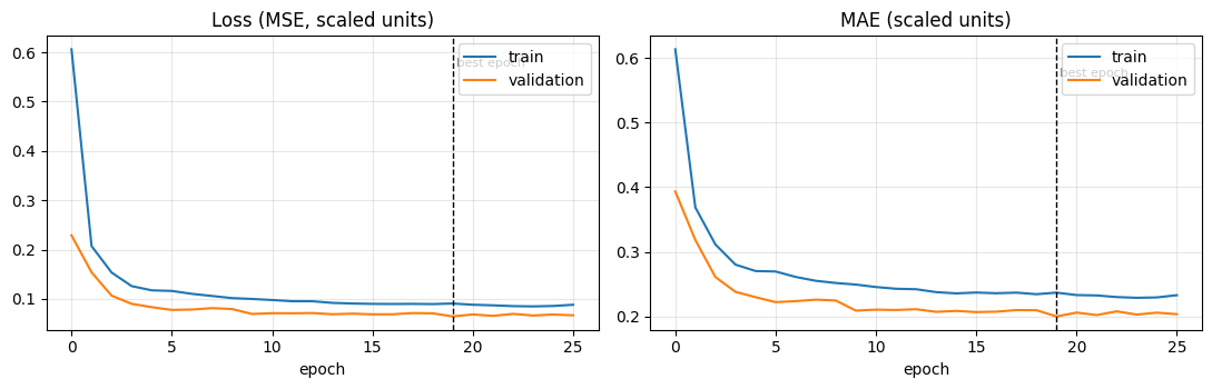
callbacks = [ keras.callbacks.EarlyStopping(monitor="val_loss", patience=6, restore_best_weights=True), keras.callbacks.ReduceLROnPlateau(monitor="val_loss", factor=0.5, patience=3, min_lr=1e-5),]model = build_model(units=64, dropout=0.2)history = model.fit( X_train, y_train, validation_data=(X_val, y_val), epochs=40, batch_size=128, shuffle=True, callbacks=callbacks, verbose=0, # set to 1 to watch it train)print(f"stopped after {len(history.history['loss'])} epochs")print(f"best val_loss: {min(history.history['val_loss']):.5f}")
WARNING:absl:At this time, the v2.11+ optimizer `tf.keras.optimizers.Adam` runs slowly on M1/M2 Macs, please use the legacy Keras optimizer instead, located at `tf.keras.optimizers.legacy.Adam`.
WARNING:absl:There is a known slowdown when using v2.11+ Keras optimizers on M1/M2 Macs. Falling back to the legacy Keras optimizer, i.e., `tf.keras.optimizers.legacy.Adam`.
stopped after 26 epochs
best val_loss: 0.06440
Learning curves: the overfitting diagnostic
Read this plot like a doctor reads an X-ray:
train ↓, val ↓, curves close together → healthy, maybe undertrained
train ↓, val flat or ↑, gap widening → overfitting; add regularization or stop earlier
both flat and high → underfitting; more capacity, longer lookback, or higher learning rate
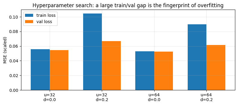
Tuning is not optional, but it also does not have to be elaborate. A tiny grid over the knobs that actually matter: capacity (units) and regularization strength (dropout): teaches the core discipline:
Select on validation loss. The test set is not a selection tool.
Every time you look at the test set to make a decision, you spend a little of its integrity. Look once, at the end.
WARNING:absl:At this time, the v2.11+ optimizer `tf.keras.optimizers.Adam` runs slowly on M1/M2 Macs, please use the legacy Keras optimizer instead, located at `tf.keras.optimizers.legacy.Adam`.
WARNING:absl:There is a known slowdown when using v2.11+ Keras optimizers on M1/M2 Macs. Falling back to the legacy Keras optimizer, i.e., `tf.keras.optimizers.legacy.Adam`.
WARNING:absl:At this time, the v2.11+ optimizer `tf.keras.optimizers.Adam` runs slowly on M1/M2 Macs, please use the legacy Keras optimizer instead, located at `tf.keras.optimizers.legacy.Adam`.
WARNING:absl:There is a known slowdown when using v2.11+ Keras optimizers on M1/M2 Macs. Falling back to the legacy Keras optimizer, i.e., `tf.keras.optimizers.legacy.Adam`.
WARNING:absl:At this time, the v2.11+ optimizer `tf.keras.optimizers.Adam` runs slowly on M1/M2 Macs, please use the legacy Keras optimizer instead, located at `tf.keras.optimizers.legacy.Adam`.
WARNING:absl:There is a known slowdown when using v2.11+ Keras optimizers on M1/M2 Macs. Falling back to the legacy Keras optimizer, i.e., `tf.keras.optimizers.legacy.Adam`.
WARNING:absl:At this time, the v2.11+ optimizer `tf.keras.optimizers.Adam` runs slowly on M1/M2 Macs, please use the legacy Keras optimizer instead, located at `tf.keras.optimizers.legacy.Adam`.
WARNING:absl:There is a known slowdown when using v2.11+ Keras optimizers on M1/M2 Macs. Falling back to the legacy Keras optimizer, i.e., `tf.keras.optimizers.legacy.Adam`.
labels = [f"u={r['units']}\nd={r['dropout']}"for r in results]xs = np.arange(len(results))plt.figure(figsize=(8, 3.6))plt.bar(xs -0.18, [r["train_loss"] for r in results], width=0.36, label="train loss")plt.bar(xs +0.18, [r["val_loss"] for r in results], width=0.36, label="val loss")plt.xticks(xs, labels)plt.ylabel("MSE (scaled)")plt.title("Hyperparameter search: a large train/val gap is the fingerprint of overfitting")plt.legend(); plt.tight_layout(); plt.show()
Step 9: Evaluate on the test set (once)
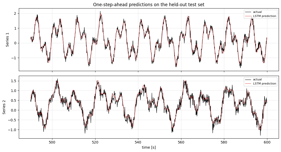
Take the configuration the validation set chose, and finally look at the held-out future.
Two sanity checks matter more than the raw number:
Did we beat the persistence baseline? If not, the LSTM has learned nothing useful.
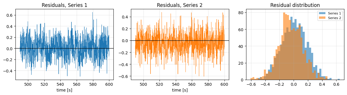
Do the residuals look like noise? Structure in the residuals means signal the model missed.
final_model = best_cfg["model"] # already restored to its best-epoch weightspred_scaled = final_model.predict(X_test, verbose=0)pred = unscale(pred_scaled)truth = unscale(y_test)lstm_rmse = rmse(truth, pred)base_rmse = rmse(truth, unscale(X_test[:, -1, :]))print(f"{'model':<24}{'RMSE':>10}{'MAE':>10}")print(f"{'persistence baseline':<24}{base_rmse:>10.4f}{mae(truth, unscale(X_test[:, -1, :])):>10.4f}")print(f"{'LSTM':<24}{lstm_rmse:>10.4f}{mae(truth, pred):>10.4f}")print(f"\nimprovement over baseline: {100* (1- lstm_rmse / base_rmse):.1f}%")for i, name inenumerate(["Series 1", "Series 2"]):print(f" {name}: RMSE {rmse(truth[:, i], pred[:, i]):.4f}")
model                         RMSE       MAE
persistence baseline        0.2243    0.1777
LSTM                        0.1754    0.1405

improvement over baseline: 21.8%
  Series 1: RMSE 0.1769
  Series 2: RMSE 0.1739
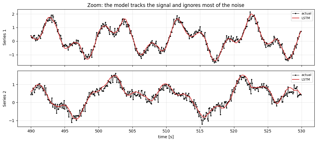
# Zoom: 40 seconds of test data, so the fit is actually visible.zs =slice(0, 400)fig, axes = plt.subplots(2, 1, sharex=True, figsize=(11, 5))for i, (ax, name) inenumerate(zip(axes, ["Series 1", "Series 2"])): ax.plot(t_test[zs], truth[zs, i], "o-", ms=2, lw=0.8, color="k", label="actual") ax.plot(t_test[zs], pred[zs, i], lw=1.4, color="C3", label="LSTM") ax.set_ylabel(name); ax.legend(fontsize=8)axes[0].set_title("Zoom: the model tracks the signal and ignores most of the noise")axes[1].set_xlabel("time [s]")plt.tight_layout(); plt.show()
resid = truth - predfig, axes = plt.subplots(1, 3, figsize=(12, 3.4))axes[0].plot(t_test, resid[:, 0], lw=0.6); axes[0].axhline(0, color="k", lw=1)axes[0].set_title("Residuals, Series 1"); axes[0].set_xlabel("time [s]")axes[1].plot(t_test, resid[:, 1], lw=0.6, color="C1"); axes[1].axhline(0, color="k", lw=1)axes[1].set_title("Residuals, Series 2"); axes[1].set_xlabel("time [s]")axes[2].hist(resid[:, 0], bins=40, alpha=0.6, label="Series 1")axes[2].hist(resid[:, 1], bins=40, alpha=0.6, label="Series 2")axes[2].set_title("Residual distribution"); axes[2].legend(fontsize=8)plt.tight_layout(); plt.show()print("residual std :", resid.std(axis=0).round(3), " (observation noise was", noise_std, ")")print("A residual std near the noise floor means the model has extracted essentially all")print("the learnable structure: you cannot predict the noise.")
residual std : [0.177 0.169]    (observation noise was 0.15 )
A residual std near the noise floor means the model has extracted essentially all
the learnable structure: you cannot predict the noise.
Step 10: Forecasting into the future: recursive multi-step
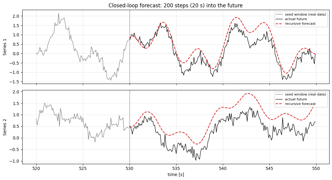
Everything above is one-step-ahead, where the model always gets a window of real data. That is not forecasting; that is nowcasting.
To predict \(H\) steps into the future you go closed-loop: predict one step, append the prediction to the window, slide, predict again. The model now consumes its own output.
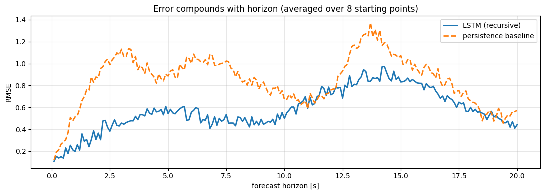
This is where it gets hard. Each prediction carries error, and that error becomes input to the next prediction. Errors compound. The forecast horizon at which an LSTM stops beating persistence is the number that actually matters in production: and it is usually shorter than people hope.
def recursive_forecast(model, seed_window, n_steps):"""seed_window: (lookback, features) scaled. Returns (n_steps, features) scaled.""" window = seed_window.copy() out = []for _ inrange(n_steps): p = model.predict(window[np.newaxis, ...], verbose=0)[0] # (features,) out.append(p) window = np.vstack([window[1:], p]) # drop oldest, append the PREDICTIONreturn np.array(out)H =200# forecast 200 steps = 20 seconds aheadstart =500# start somewhere inside the test setseed = test[start - LOOKBACK : start] # the last real data the model is allowed to seefc_scaled = recursive_forecast(final_model, seed, H)fc = unscale(fc_scaled)actual_future = unscale(test[start : start + H])t_seed = t[n_train + n_val + start - LOOKBACK : n_train + n_val + start]t_future = t[n_train + n_val + start : n_train + n_val + start + H]
# How fast does the error grow with the horizon? Average over many starting points.starts = np.arange(LOOKBACK, len(test) - H, 120)errors = np.zeros((len(starts), H))persist_errors = np.zeros((len(starts), H))for j, s inenumerate(starts): f = unscale(recursive_forecast(final_model, test[s - LOOKBACK : s], H)) a = unscale(test[s : s + H]) last_value = unscale(test[s -1 : s]) # persistence: hold the last value errors[j] = np.sqrt(((f - a) **2).mean(axis=1)) persist_errors[j] = np.sqrt(((last_value - a) **2).mean(axis=1))plt.figure()plt.plot(np.arange(1, H +1) / fs, errors.mean(axis=0), lw=2, label="LSTM (recursive)")plt.plot(np.arange(1, H +1) / fs, persist_errors.mean(axis=0), lw=2, ls="--", label="persistence baseline")plt.xlabel("forecast horizon [s]"); plt.ylabel("RMSE")plt.title(f"Error compounds with horizon (averaged over {len(starts)} starting points)")plt.legend(); plt.tight_layout(); plt.show()crossings = np.where(errors.mean(axis=0) > persist_errors.mean(axis=0))[0]iflen(crossings):print(f"The LSTM stops beating persistence at ~{(crossings[0] +1) / fs:.1f} s ahead.")else:print("The LSTM beats persistence across the entire tested horizon.")
The LSTM stops beating persistence at ~10.7 s ahead.