import numpy as np
import pandas as pd
import matplotlib.pyplot as plt
from scipy.interpolate import interp1d, CubicSpline, PchipInterpolator

plt.rcParams.update({
    "figure.dpi": 110,
    "axes.grid": True,
    "grid.alpha": 0.3,
    "axes.spines.top": False,
    "axes.spines.right": False,
    "font.size": 11,
})

TRUE   = "#9e9e9e"   # the (normally unknown) underlying signal
OBS    = "#1f4e79"   # observed points
FILL = "#d1495b" # interpolated curve / filled pointsInterpolating Missing Values in Time Series
Part 1: Univariate: what is interpolation?
1.1 Setup
A 20-step series. We know the true generating function (in real life you never do: that is the point of the exercise), and we knock out 5 of the 20 points, including two consecutive gaps. Consecutive gaps matter: they are where interpolation methods disagree most.
The observations also carry a little measurement noise, as real data do. This is worth pausing on, because it sharpens the definition: an interpolant passes exactly through the observed points, noise and all. Interpolation reproduces noise; it does not filter it. (Filtering it is smoothing: a different job.) We will score each method against the clean signal at the missing steps, since recovering the signal is what we actually want.
rng = np.random.default_rng(0)

def f_true(t):
    # The underlying signal. Unknown in practice; here it is our ground truth.
    return np.sin(0.55 * t) + 0.06 * t

t_all   = np.arange(20)                                    # the temporal mesh: 20 time steps
y_all   = f_true(t_all) + rng.normal(0, 0.08, t_all.size)  # observations = signal + measurement noise

missing = np.array([4, 5, 11, 15, 16])          # 5 missing steps, two of them consecutive pairs
obs     = np.setdiff1d(t_all, missing)          # the 15 steps we actually observe

t_obs, y_obs = t_all[obs], y_all[obs]           # what we actually have
t_mis        = t_all[missing]
y_mis        = f_true(t_mis)                    # clean signal at the holes: the target we score against

t_dense = np.linspace(0, 19, 500)     # fine grid, used only to *draw* the interpolants

print(f"observed: {len(t_obs)} points   missing: {len(t_mis)} points -> {t_mis}")
observed: 15 points missing: 5 points -> [ 4 5 11 15 16]def show(ax, f_interp=None, title="", ylim=None):
# One consistent picture: truth, observed points, gaps, and the fitted interpolant.
ax.plot(t_dense, f_true(t_dense), color=TRUE, lw=1.2, ls="--", label="true signal (unknown)")
if f_interp is not None:
ax.plot(t_dense, f_interp(t_dense), color=FILL, lw=2.0, label="interpolant $f$")
ax.scatter(t_mis, f_interp(t_mis), color=FILL, s=70, zorder=5,
marker="X", label="imputed value")
ax.scatter(t_obs, y_obs, color=OBS, s=45, zorder=6, label="observed")
for t in t_mis: # mark the holes
ax.axvline(t, color="k", alpha=0.08, lw=8)
ax.set_title(title, fontsize=11)
ax.set_xlabel("time step"); ax.set_ylabel("y")
if ylim: ax.set_ylim(*ylim)
return ax
fig, ax = plt.subplots(figsize=(9, 3.4))
show(ax, None, "The problem: 5 of 20 points are missing (grey bands)")
ax.legend(loc="upper left", fontsize=9, ncol=3)
plt.tight_layout(); plt.show()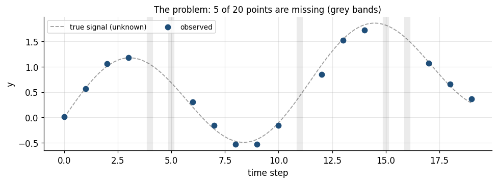
1.2 Zero-order hold: forward fill (LOCF)
The simplest possible assumption: nothing changed since the last observation.
\[f(t) = y_i \quad \text{for } t_i \le t < t_{i+1}\]
- Piecewise constant, discontinuous at each knot.
- Causal: it uses only the past. That is its real virtue: for a live model or a backtest, forward fill is the only fill that cannot leak the future into a feature.
- Systematically lags the signal and flattens variance across the gap.
f_ffill = interp1d(t_obs, y_obs, kind="previous", bounds_error=False,
                   fill_value=(y_obs[0], y_obs[-1]))

fig, ax = plt.subplots(figsize=(9, 3.4))
show(ax, f_ffill, "Forward fill (zero-order hold): flat steps, lags the true signal")
ax.legend(loc="upper left", fontsize=9, ncol=2)
plt.tight_layout(); plt.show()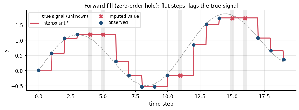
1.3 Linear interpolation
Connect consecutive observations with straight lines. On the interval \([t_i,\,t_{i+1}]\):
\[f(t) = y_i + \big(y_{i+1}-y_i\big)\,\frac{t - t_i}{t_{i+1} - t_i}\]
- \(C^0\): continuous, but the slope jumps at every knot (visible kinks).
- No overshoot: \(f(t)\) always stays between \(y_i\) and \(y_{i+1}\). This is a strong safety property.
- Accuracy on a gap of width \(h\): the error is \(O(h^2 \max|f''|)\): it is exact for straight lines and degrades with curvature. So it is fine for one missing point, worse for a long gap.
This is the workhorse. It is pandas’ default and it is the right first choice most of the time.
f_lin = interp1d(t_obs, y_obs, kind="linear")

fig, ax = plt.subplots(figsize=(9, 3.4))
show(ax, f_lin, "Linear: chords between neighbours. Note the error grows on the 2-step gaps.")
ax.legend(loc="upper left", fontsize=9, ncol=2)
plt.tight_layout(); plt.show()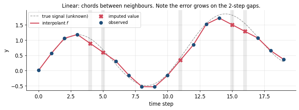
1.4 Global polynomial: the cautionary tale
Through \(n\) points there is exactly one polynomial of degree \(n-1\) (the Lagrange interpolant). Here \(n = 15\), so degree 14. It passes through every observation perfectly and is infinitely smooth.
It is also unusable on real data, and it is worth being precise about why, because the usual one-word answer (“Runge”) is only half of it.
The interpolant depends on the data through the Lebesgue constant \(\Lambda_n\): a perturbation of the observations of size \(\varepsilon\) can move the interpolant by as much as \(\Lambda_n \varepsilon\). For equispaced nodes \(\Lambda_n\) grows exponentially, roughly \(2^n / (n\log n)\):
\[\Lambda_5 \approx 2, \qquad \Lambda_{10} \approx 18, \qquad \Lambda_{15} \approx 283, \qquad \Lambda_{20} \approx 5900\]
For our 15 nodes \(\Lambda_n \approx 371\). So our modest noise of \(\sigma = 0.08\) can be amplified into swings of order \(371 \times 0.08 \approx 30\). The polynomial is not bending to follow the signal; it is bending to chase the noise, and it must do so with a single global function that cannot bend in one place without flailing everywhere else.
Aside, and a caveat on the demo below. On a noiseless analytic signal like our sine, the degree-14 interpolant is actually superb: it would score near-zero error here. Runge’s phenomenon in its strict sense needs a function with a singularity near the interval (the classic \(1/(1+25x^2)\)). What kills high-degree polynomial interpolation on data is the exponential noise amplification above. That is the failure mode you will actually meet, so it is the one shown.
The lesson that motivates splines: don’t fit one high-degree polynomial globally. Fit many low-degree polynomials locally, and glue them together smoothly. Their Lebesgue constants stay bounded as \(n\) grows.
coeffs   = np.polyfit(t_obs, y_obs, deg=len(t_obs) - 1)   # degree 14
f_poly   = np.poly1d(coeffs)

fig, axes = plt.subplots(1, 2, figsize=(11, 3.6))
show(axes[0], f_poly, "Degree-14 polynomial (zoomed to the data range)", ylim=(-2, 3))
show(axes[1], f_poly, "...the same curve, unzoomed: it chases the noise")
axes[0].legend(loc="upper left", fontsize=8)
plt.tight_layout(); plt.show()

print("value imputed at t=16 :", f_poly(16).round(2), " | truth:", f_true(16).round(2))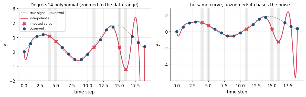
value imputed at t=16 : -1.22 | truth: 1.541.5 Cubic spline
Fit a separate cubic on each interval and force the pieces to agree at the knots. On \([t_i,\,t_{i+1}]\):
\[S_i(t) = a_i + b_i(t-t_i) + c_i(t-t_i)^2 + d_i(t-t_i)^3\]
The coefficients are pinned down by requiring, at every interior knot:
\[S_{i-1}(t_i) = S_i(t_i) = y_i, \qquad S_{i-1}'(t_i) = S_i'(t_i), \qquad S_{i-1}''(t_i) = S_i''(t_i)\]
i.e. the curve is \(C^2\): continuous in value, slope, and curvature. Two conditions remain; the natural spline sets \(S''=0\) at both ends. Solving gives a small tridiagonal linear system.
- Very accurate for smooth signals: error is \(O(h^4)\), versus \(O(h^2)\) for linear.
- Degree stays at 3 no matter how many points there are, so no Runge blow-up.
- But it can overshoot. \(C^2\) smoothness forces the curve to “carry momentum” through a gap, so it can shoot past the neighbouring values: a real hazard for bounded quantities (a rate that must stay positive, a share that must stay in \([0,1]\)).
f_spline = CubicSpline(t_obs, y_obs, bc_type="natural")

fig, ax = plt.subplots(figsize=(9, 3.4))
show(ax, f_spline, "Natural cubic spline: smooth ($C^2$) and accurate here: but watch for overshoot")
ax.legend(loc="upper left", fontsize=9, ncol=2)
plt.tight_layout(); plt.show()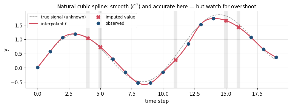
1.6 PCHIP: shape-preserving cubic
Same piecewise-cubic idea, but the derivative at each knot is chosen, not solved for, using a weighted-harmonic-mean rule on the neighbouring slopes \(\Delta_i = (y_{i+1}-y_i)/(t_{i+1}-t_i)\):
\[d_i = 0 \ \ \text{if } \Delta_{i-1}\Delta_i \le 0 \qquad\text{(a local extremum: flatten it)}\]
This gives up \(C^2\) (PCHIP is only \(C^1\)) and buys a guarantee: the interpolant is monotone wherever the data are monotone, so it never overshoots.
A good default for economic and financial series, which are full of level shifts and kinks that a \(C^2\) spline will ring around.
f_pchip = PchipInterpolator(t_obs, y_obs)

fig, ax = plt.subplots(figsize=(9, 3.4))
show(ax, f_pchip, "PCHIP: cubic, but shape-preserving: no overshoot, slightly flatter at the peaks")
ax.legend(loc="upper left", fontsize=9, ncol=2)
plt.tight_layout(); plt.show()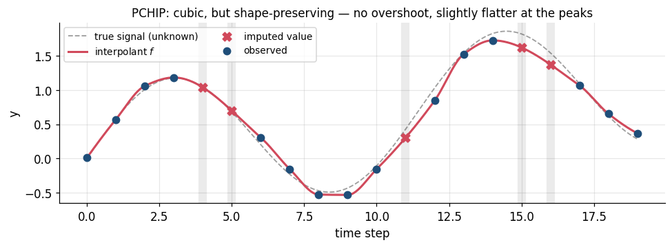
1.7 Side by side, and which one was actually right
Because this is synthetic data we know the truth at the missing points, so we can score each method. Reported error is the mean absolute error evaluated only at the 5 missing time steps: the only places the methods differ.
methods = {
    "Forward fill":    f_ffill,
    "Nearest":         interp1d(t_obs, y_obs, kind="nearest"),
    "Linear":          f_lin,
    "Cubic spline":    f_spline,
    "PCHIP":           f_pchip,
    "Poly (deg 14)":   f_poly,
}

fig, axes = plt.subplots(2, 3, figsize=(13.5, 6.4), sharex=True)
for ax, (name, f) in zip(axes.ravel(), methods.items()):
    show(ax, f, name, ylim=(-2.0, 3.0))
axes[0, 0].legend(loc="upper left", fontsize=7.5)
fig.suptitle("Same 15 observations, six different assumptions about the gaps", y=1.00)
plt.tight_layout(); plt.show()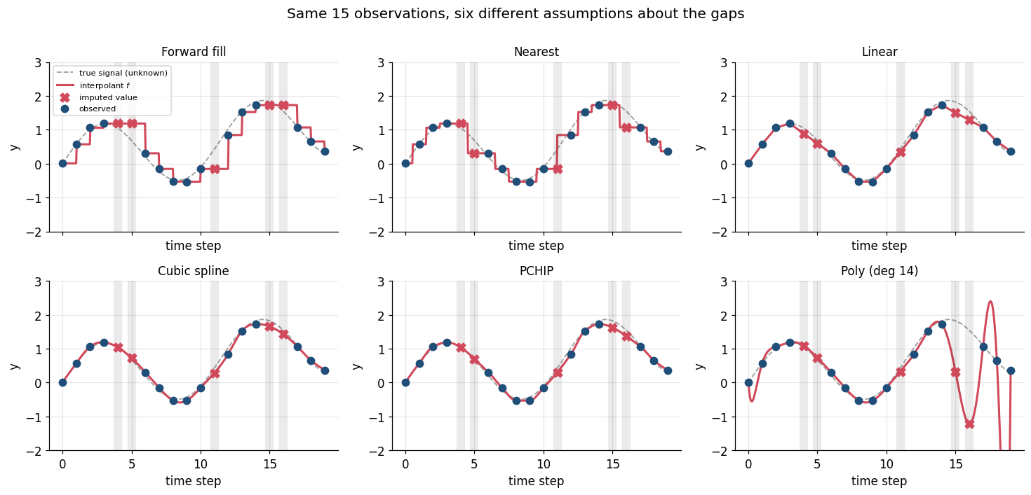
scores = pd.DataFrame({
    "MAE at gaps":  {n: np.abs(f(t_mis) - y_mis).mean()  for n, f in methods.items()},
    "Max error":    {n: np.abs(f(t_mis) - y_mis).max()   for n, f in methods.items()},
}).sort_values("MAE at gaps")

display(scores.style.format("{:.3f}").background_gradient(cmap="Reds", subset=["MAE at gaps"]))

fig, ax = plt.subplots(figsize=(7, 3))
s = scores["MAE at gaps"]
ax.barh(s.index[::-1], s.values[::-1], color=FILL, alpha=0.85)
ax.set_xscale("log"); ax.set_xlabel("MAE at the missing steps (log scale)")
ax.set_title("Smooth signal + a little noise -> the C² spline wins, the polynomial melts down")
plt.tight_layout(); plt.show()| MAE at gaps | Max error | |
|---|---|---|
| Cubic spline | 0.096 | 0.165 |
| PCHIP | 0.104 | 0.198 |
| Linear | 0.178 | 0.314 |
| Forward fill | 0.300 | 0.584 |
| Nearest | 0.333 | 0.584 |
| Poly (deg 14) | 0.892 | 2.765 |
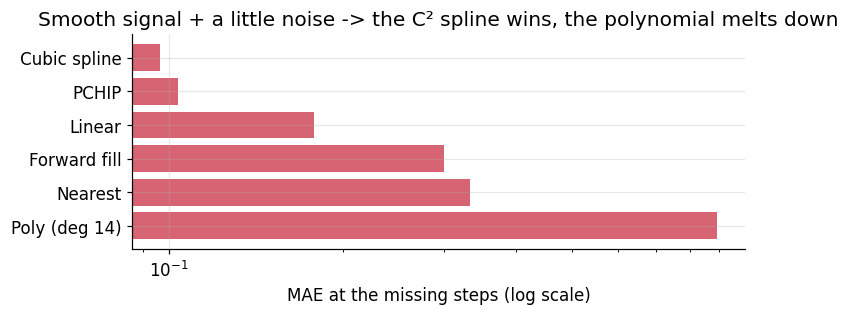
Read the ranking carefully: it is a property of this signal, not a law. The truth here is a smooth, gently-curving sinusoid, which is exactly what a cubic spline is built to reproduce, so the spline wins and PCHIP is close behind. On a series with jumps, regime shifts, or heavy noise, plain linear or PCHIP will typically beat the spline, because its \(C^2\) momentum turns into ringing. In Part 2 we will see the cubic spline finish best on one series and worst on another within the same dataset. This is why Part 2 ends with an empirical check rather than a rule of thumb.
Practical summary
| Method | Continuity | Overshoots? | Use when |
|---|---|---|---|
| Forward fill | none | no | causal features; step-like series (policy rates, ratings) |
| Linear | \(C^0\) | no | default; short gaps; when you want no surprises |
| Cubic spline | \(C^2\) | yes | genuinely smooth series; when derivatives matter |
| PCHIP | \(C^1\) | no | smooth-ish but bounded/monotone series |
| Global polynomial | \(C^\infty\) | catastrophically | never, beyond ~5 points |
Part 2: Multivariate: the standard pandas workflow
Three correlated daily economic series over ~90 days, driven by a common latent macro factor:
equity_index: an equity benchmark levelyield_10y: the 10-year government bond yield (%), mean-revertingoil_wti: crude oil spot price ($/bbl)
We generate them complete (so we retain ground truth for scoring), then punch holes in them, including several multi-day consecutive gaps and one date range where the data vendor dropped the rows entirely.
rng = np.random.default_rng(7)
n   = 90
dates = pd.date_range("2024-01-01", periods=n, freq="D")

macro = np.cumsum(rng.normal(0, 1, n)) * 0.6          # shared latent factor

equity = 4400 + 42 * macro + np.cumsum(rng.normal(0.8, 6.0, n))
oil    = 78   +  1.8 * macro + np.cumsum(rng.normal(0.0, 0.7, n))

yield10 = np.empty(n); yield10[0] = 4.20              # Ornstein-Uhlenbeck-ish mean reversion
for i in range(1, n):
    yield10[i] = yield10[i-1] + 0.08*(4.20 - yield10[i-1]) - 0.010*macro[i] + rng.normal(0, 0.035)

truth = pd.DataFrame({"equity_index": equity, "yield_10y": yield10, "oil_wti": oil}, index=dates)
truth.index.name = "date"
truth.head()| equity_index | yield_10y | oil_wti | |
|---|---|---|---|
| date | |||
| 2024-01-01 | 4400.686138 | 4.200000 | 77.692527 |
| 2024-01-02 | 4413.024812 | 4.197943 | 77.659599 |
| 2024-01-03 | 4404.877321 | 4.151590 | 77.804588 |
| 2024-01-04 | 4389.547164 | 4.220920 | 76.631442 |
| 2024-01-05 | 4378.857063 | 4.278277 | 76.034387 |
2.1 Introduce the missingness
Two flavours, and they are handled differently:
NaNs inside existing rows: the date is there, the value is not.- Missing rows entirely: a holiday shutdown where the vendor simply sent nothing. These are invisible until you put the data back on a regular mesh, and they are the classic silent bug:
.diff()and.rolling()will happily treat Jan 20 and Jan 25 as adjacent.
raw = truth.copy()

gaps = {                                    # (start_row, n_consecutive_days)
    "equity_index": [(20, 5), (61, 2)],
    "yield_10y":    [(33, 1), (44, 7)],
    "oil_wti":      [(12, 3), (55, 8), (78, 2)],
}
for col, spans in gaps.items():
    for start, length in spans:
        raw.iloc[start:start + length, raw.columns.get_loc(col)] = np.nan

dropped = pd.date_range("2024-03-04", periods=4, freq="D")   # vendor dropped these rows outright
raw = raw.drop(index=dropped)

print(f"rows on file: {len(raw)}   (calendar days spanned: {(raw.index.max()-raw.index.min()).days + 1})")
print("\nNaNs per column, as delivered:")
print(raw.isna().sum())
rows on file: 86 (calendar days spanned: 90)
NaNs per column, as delivered:
equity_index 7
yield_10y 8
oil_wti 13
dtype: int642.2 Step 1: put the data back on a regular temporal mesh
Do this first, always. asfreq reindexes onto the full calendar and materialises the dropped rows as NaN. Now all the missingness is visible in one place, and every downstream operation that assumes a fixed \(\Delta t\) is safe.
df = raw.asfreq("D")          # equivalently: raw.reindex(pd.date_range(raw.index.min(), raw.index.max(), freq="D"))

print(f"rows after asfreq: {len(df)}")
print("\nNaNs per column, once the mesh is regular:")
print(df.isna().sum())
print(f"\ntotal missing cells: {int(df.isna().sum().sum())} / {df.size}"
      f"  ({df.isna().mean().mean():.1%})")
rows after asfreq: 90
NaNs per column, once the mesh is regular:
equity_index 11
yield_10y 12
oil_wti 17
dtype: int64
total missing cells: 40 / 270 (14.8%)fig, ax = plt.subplots(figsize=(12, 2.2))
ax.imshow(df.isna().T.values, aspect="auto", cmap="Greys", interpolation="nearest",
extent=[0, len(df), len(df.columns) - 0.5, -0.5])
ax.set_yticks(range(len(df.columns))); ax.set_yticklabels(df.columns)
ax.set_xlabel("day index"); ax.set_title("Missingness map (black = NaN)")
ax.grid(False)
plt.tight_layout(); plt.show()
The four black cells that line up vertically across all three rows are the dropped vendor rows — the failure mode that asfreq just exposed.
2.3 Step 2: interpolate
The one-liner. Two arguments carry all the weight:
method="time": linear interpolation in the time coordinate, using actual timestamp spacing rather than row position. On a perfectly regular index it is identical to"linear"; the moment the index is irregular (business days, mixed frequency),"linear"is wrong and"time"is right. Make it your habit.limit_area="inside": fill only between observed values. Without it,interpolatewill happily run past the last observation and extrapolate, which is a different and far more dangerous operation. This one keyword is the guardrail.
filled = df.interpolate(method="time", limit_area="inside")

print("NaNs remaining after interpolation:")
print(filled.isna().sum())
filled.loc["2024-03-02":"2024-03-09"].round(2)      # the dropped-row window, now reconstructed
NaNs remaining after interpolation:
equity_index 0
yield_10y 0
oil_wti 0
dtype: int64| equity_index | yield_10y | oil_wti | |
|---|---|---|---|
| date | |||
| 2024-03-02 | 4075.68 | 5.27 | 60.97 |
| 2024-03-03 | 4072.36 | 5.25 | 60.96 |
| 2024-03-04 | 4069.04 | 5.24 | 60.96 |
| 2024-03-05 | 4065.71 | 5.23 | 60.96 |
| 2024-03-06 | 4062.39 | 5.22 | 60.95 |
| 2024-03-07 | 4059.07 | 5.21 | 60.95 |
| 2024-03-08 | 4055.75 | 5.20 | 60.95 |
| 2024-03-09 | 4033.12 | 5.17 | 59.03 |
Two further guardrails worth knowing, both about refusing to fill:
limit=k: fill at mostkconsecutiveNaNs. A 2-day gap in a daily series is a reasonable thing to bridge. A 3-week gap is not; interpolating it manufactures a straight line and hands your model a fabricated, artificially low-variance stretch of “data”. Set a limit and let the rest stayNaNso a later step has to make a conscious decision about it.- Edges:
limit_area="inside"deliberately leaves leading/trailingNaNs. If you must have them,.ffill()/.bfill()at least makes the extrapolation explicit and flat, rather than silently linear.
conservative = df.interpolate(method="time", limit=3, limit_area="inside")

print("NaNs left when we refuse to bridge gaps longer than 3 days:")
print(conservative.isna().sum())      # the 7- and 8-day gaps are (correctly) left alone
NaNs left when we refuse to bridge gaps longer than 3 days:
equity_index 5
yield_10y 5
oil_wti 9
dtype: int642.4 Step 3: look at it
Never ship a fill you have not plotted. Below: observed points in blue, the reconstructed segments in red, gap windows shaded.
def nan_spans(mask):
    # Yield (start, end) index for each run of True in a boolean array.
    idx = np.flatnonzero(mask)
    if idx.size == 0: return
    for grp in np.split(idx, np.flatnonzero(np.diff(idx) != 1) + 1):
        yield grp[0], grp[-1]

fig, axes = plt.subplots(3, 1, figsize=(12, 8), sharex=True)
for ax, col in zip(axes, df.columns):
    was_nan = df[col].isna().values
    ax.plot(filled.index, filled[col], color=FILL, lw=1.6, zorder=2, label="interpolated series")
    ax.plot(df.index,     df[col],     color=OBS,  lw=1.6, zorder=3, label="observed")
    ax.scatter(df.index[was_nan], filled[col].values[was_nan],
               color=FILL, s=26, zorder=4, label="imputed values")
    for a, b in nan_spans(was_nan):
        ax.axvspan(df.index[a], df.index[b], color="k", alpha=0.07, zorder=1)
    ax.set_ylabel(col); ax.set_title(f"{col} :  {was_nan.sum()} days imputed", loc="left", fontsize=10)
axes[0].legend(loc="upper left", fontsize=9, ncol=3)
axes[-1].set_xlabel("date")
plt.tight_layout(); plt.show()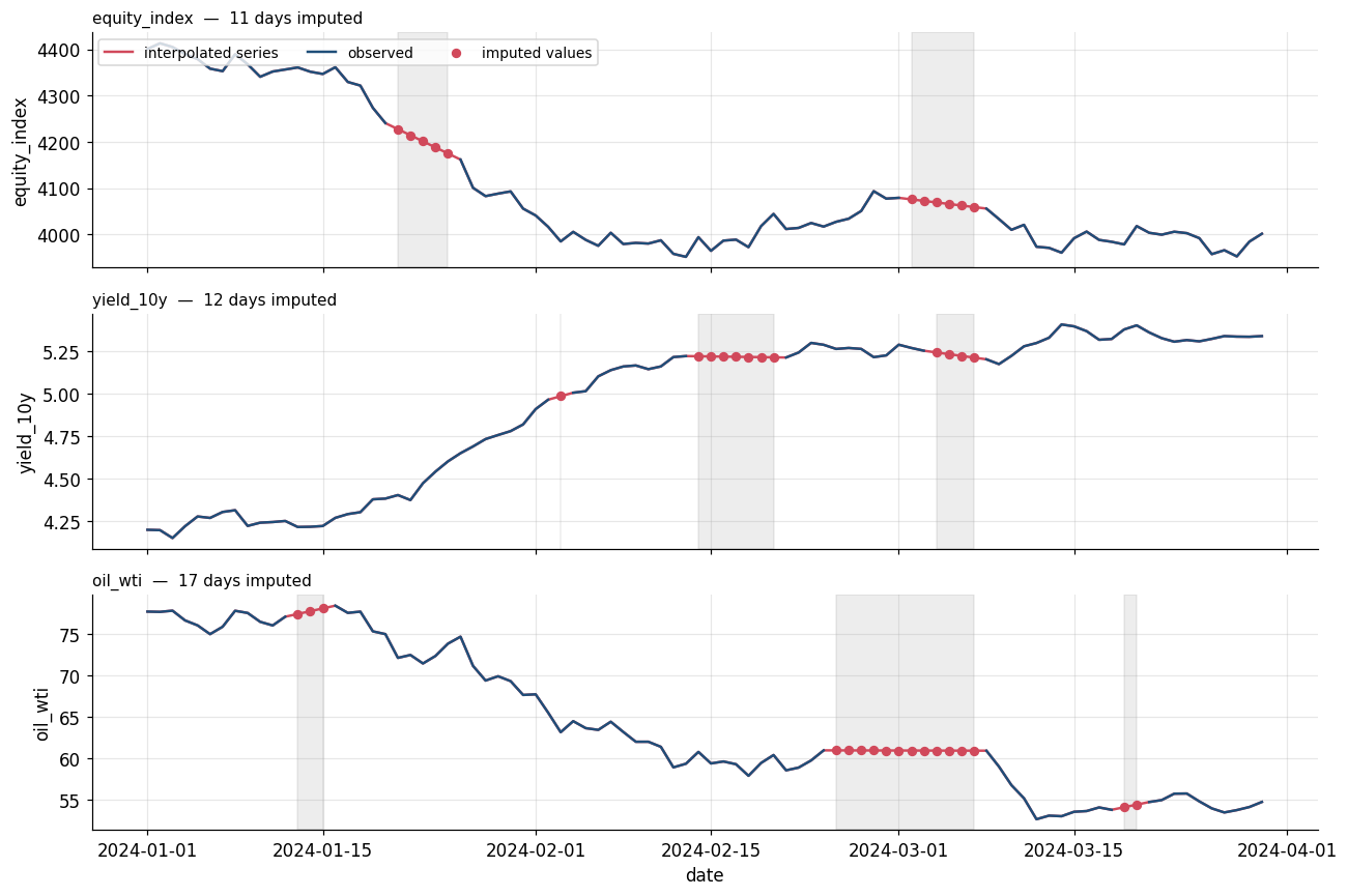
The long gaps are immediately recognisable as straight lines, and that is the honest picture of what linear interpolation does: across an 8-day hole it asserts a constant drift and zero volatility. The reconstruction is plausible in level and badly wrong in texture.
2.5 Step 4: choose the method empirically, don’t guess
We have ground truth here, so we can score directly. In a real project you get the same answer by masking values you actually observe, interpolating, and scoring against what you hid: same code, and it is the only defensible way to pick a method.
candidates = {
    "ffill":         lambda d: d.ffill(),
    "linear/time":   lambda d: d.interpolate(method="time",  limit_area="inside"),
    "nearest":       lambda d: d.interpolate(method="nearest", limit_area="inside"),
    "cubic spline":  lambda d: d.interpolate(method="spline", order=3, limit_area="inside"),
    "pchip":         lambda d: d.interpolate(method="pchip", limit_area="inside"),
}

mask  = df.isna() & truth.reindex(df.index).notna()    # cells we hid and can score
tru   = truth.reindex(df.index)

rows = {}
for name, fn in candidates.items():
    out = fn(df)
    err = (out - tru).abs()[mask]
    rows[name] = err.mean()                            # MAE per column, over imputed cells only
mae = pd.DataFrame(rows).T

display(mae.style.format("{:.3f}").background_gradient(cmap="Reds", axis=0))| equity_index | yield_10y | oil_wti | |
|---|---|---|---|
| ffill | 49.333 | 0.029 | 0.728 |
| linear/time | 25.068 | 0.019 | 0.787 |
| nearest | 31.473 | 0.021 | 0.747 |
| cubic spline | 45.233 | 0.112 | 0.605 |
| pchip | 28.885 | 0.019 | 0.798 |
fig, axes = plt.subplots(1, 3, figsize=(13, 3.4))
for ax, col in zip(axes, mae.columns):
    s = mae[col].sort_values()
    ax.barh(s.index[::-1], s.values[::-1], color=FILL, alpha=0.85)
    ax.set_title(col, fontsize=10); ax.set_xlabel("MAE on imputed cells")
fig.suptitle("Best method is series-dependent: score it, don't assume it", y=1.03)
plt.tight_layout(); plt.show()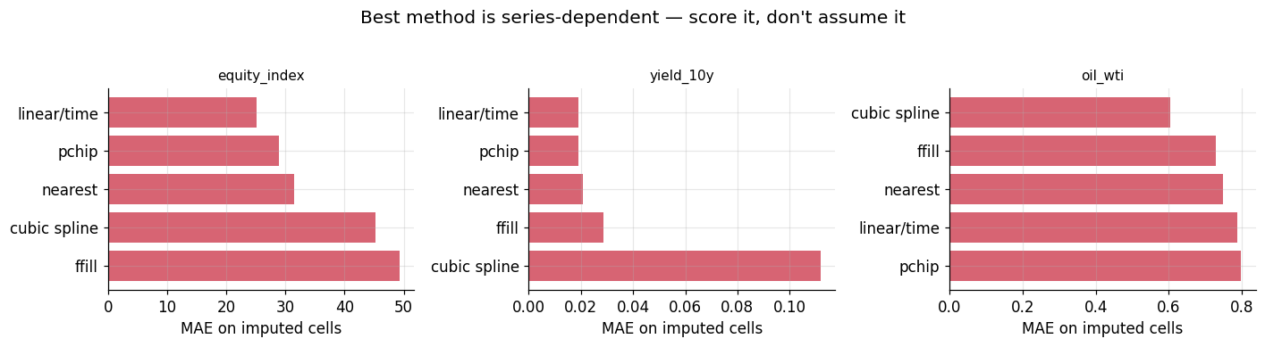
Look at what the table actually says, because it is more interesting than a tidy rule:
- No method wins everywhere.
linear/timetakesequity_indexandyield_10y(withpchipessentially tied on the latter), while the cubic spline winsoil_wtioutright. - The spline is the high-variance choice. It is the best method on
oil_wtiand, onyield_10y, roughly six times worse than linear: the worst of the five. Its flexibility is exactly what lets it win when there is real curvature to exploit and blow up when there is not. Across a long gap it carries momentum, and on a noisy mean-reverting series that momentum is ringing. ffillis worst onequity_indexby a wide margin, which is what a flat line through a five-day drift in a trending series should cost you. It is still the right choice if the feature must be causal: you are knowingly buying accuracy with lookahead-safety.
So the cubic spline’s clean victory in Part 1 does not transfer, and it does not even transfer across three columns of a single dataframe. Score it; don’t assume it.
2.6 What interpolation does not do
Filling a gap is not the same as recovering the data. Three consequences to keep in front of you:
- It fabricates smoothness. Interpolated stretches have near-zero high-frequency variance. Any statistic sensitive to that: volatility, autocorrelation at short lags, the spectrum: is biased by exactly the cells you filled. Compute those on the observed subset, or account for it.
- Most methods are not causal. Linear, spline, and PCHIP all use the value after the gap. In a backtest or a live feature pipeline, that is lookahead leakage. Forward fill is the causal choice, and this is the reason to reach for it despite its accuracy being worse.
- It ignores the other columns. We filled
oil_wtiusing onlyoil_wti, even though all three series share a common macro factor and are strongly correlated: information we simply threw away.
That third point is the natural next topic: multivariate imputation, which fills a gap in one series using the contemporaneous values of the others. The standard tools are sklearn.impute.IterativeImputer (MICE: regress each column on the rest, iterate) and state-space / Kalman smoothing (statsmodels), which is the principled choice for time series because it models the temporal dynamics and the cross-correlation jointly, and gives you uncertainty bands on the filled values rather than a single confident-looking line.
print(f"Correlation of daily changes: the structure single-column interpolation ignores:\n")
print(truth.diff().corr().round(2))
Correlation of daily changes — the structure single-column interpolation ignores:
equity_index yield_10y oil_wti
equity_index 1.00 -0.18 0.79
yield_10y -0.18 1.00 -0.22
oil_wti 0.79 -0.22 1.00