temp: [20 22 25 24 21 19 18 20 23 26 28 27]
shape: (12,)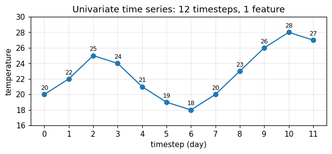
Deep learning models for sequences (RNNs, LSTMs, GRUs, 1D CNNs, Transformers) almost always expect a rank-3 tensor:
(samples, timesteps, features)The whole job of data preparation is turning raw sequential data into that shape. This notebook does it twice:
Everything is a tiny toy example so the shapes stay readable.
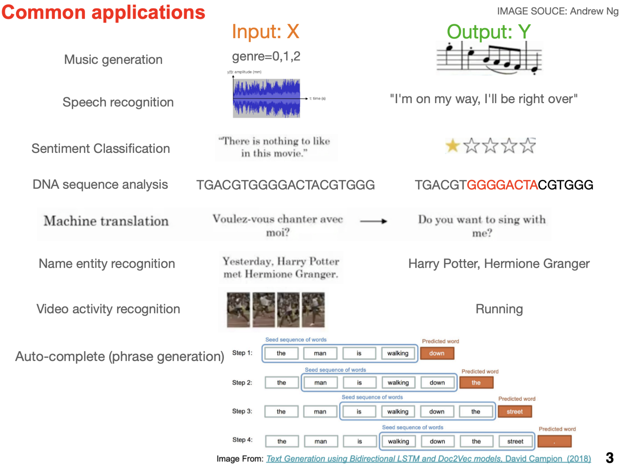
The importance of auto or cross-correlation in data
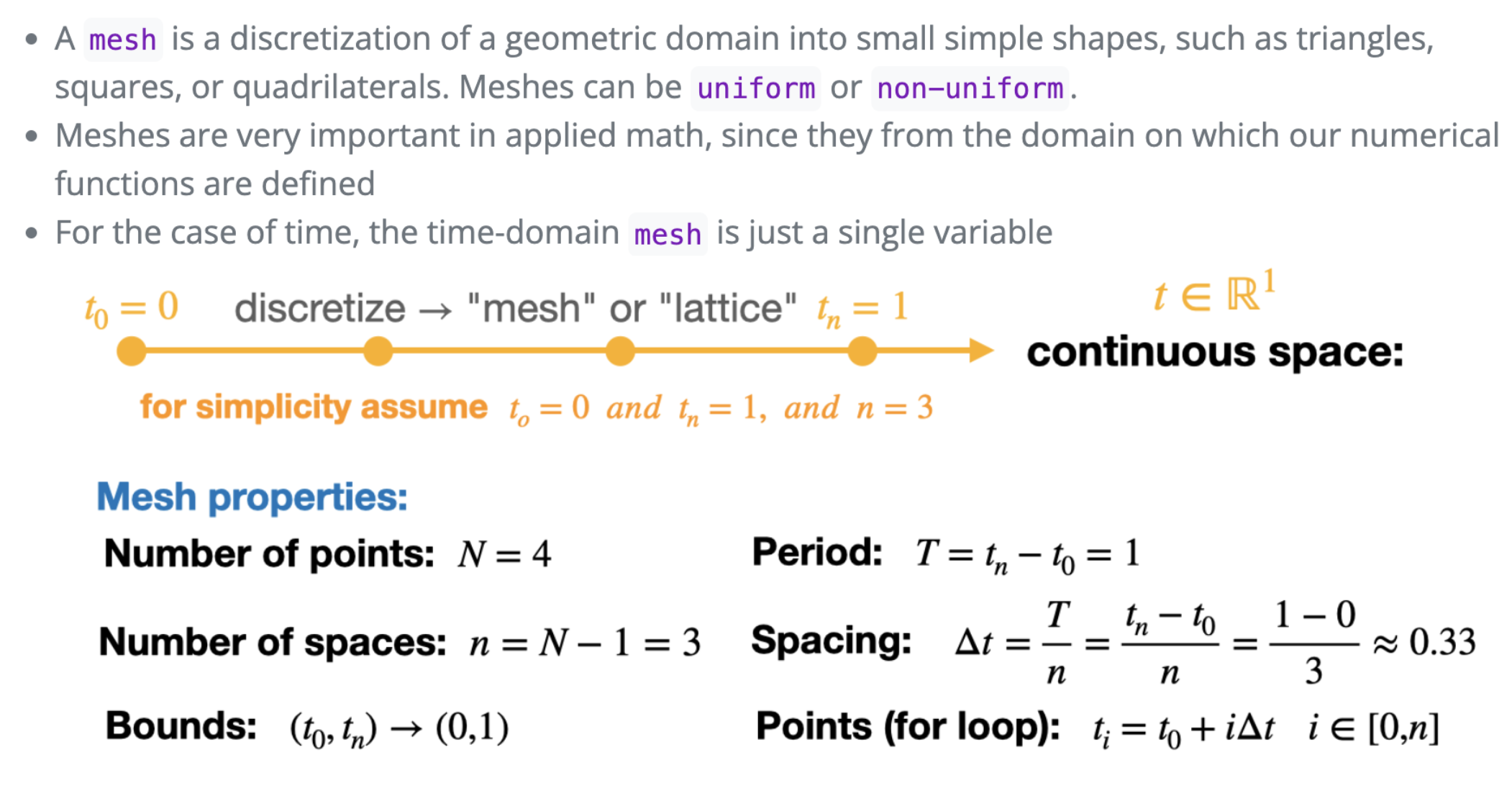
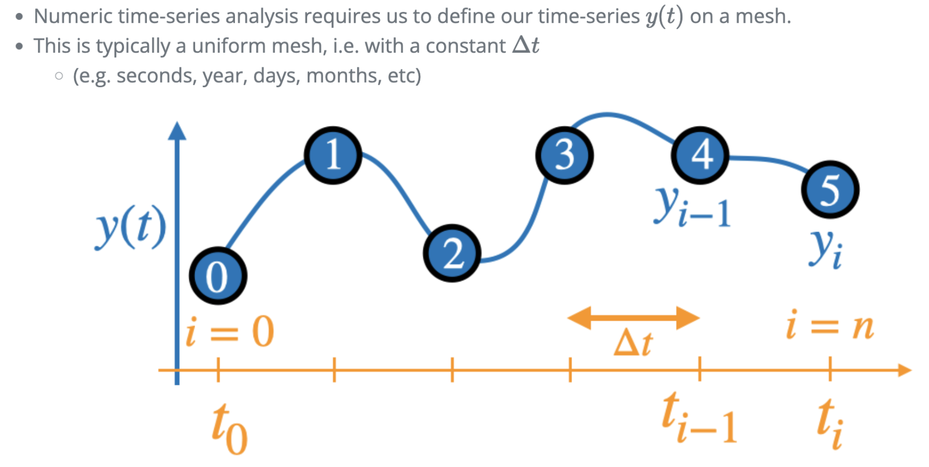
(samples, timesteps, features) so the order axis becomes explicit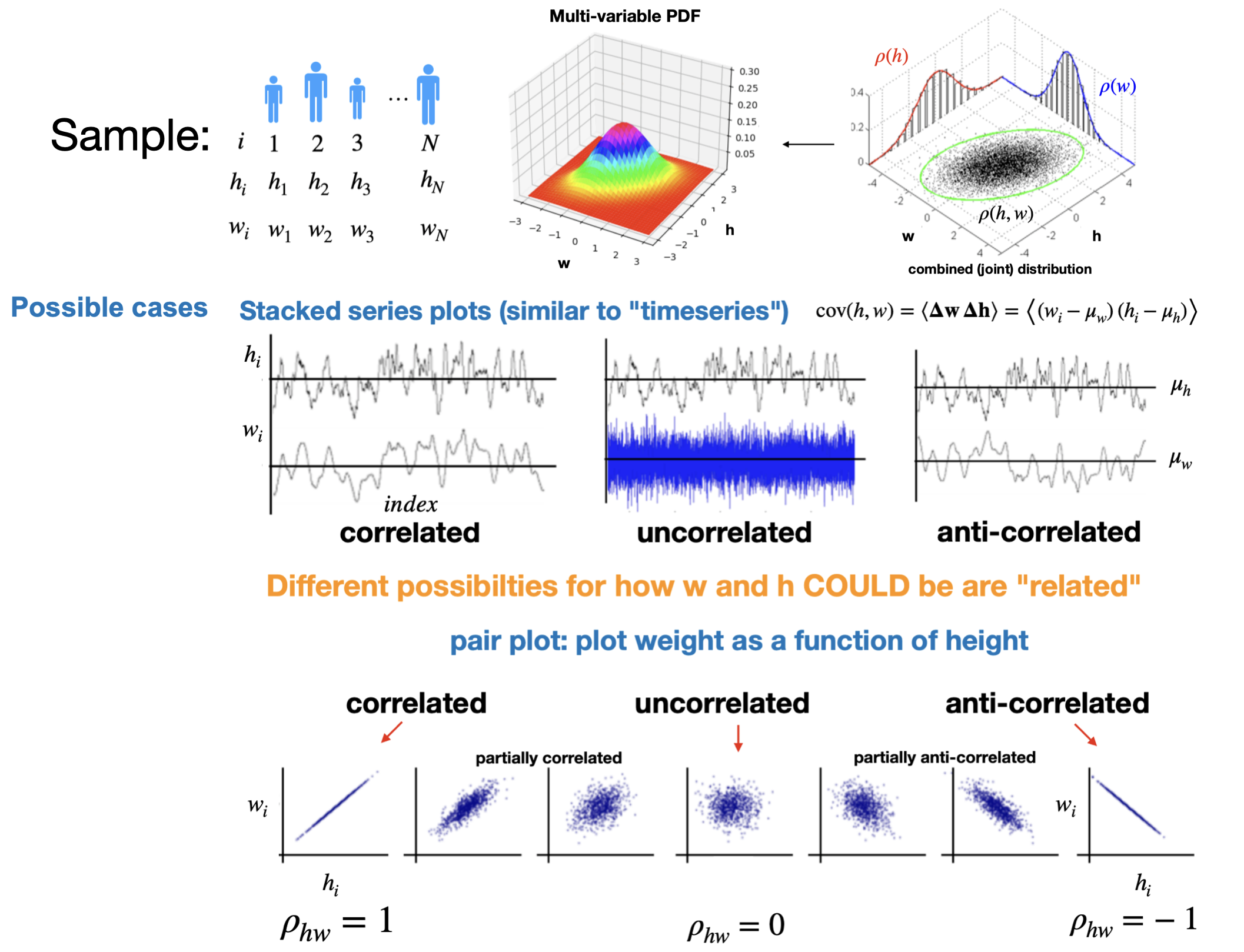
Auto-correlation Internal correlation (self correlation)
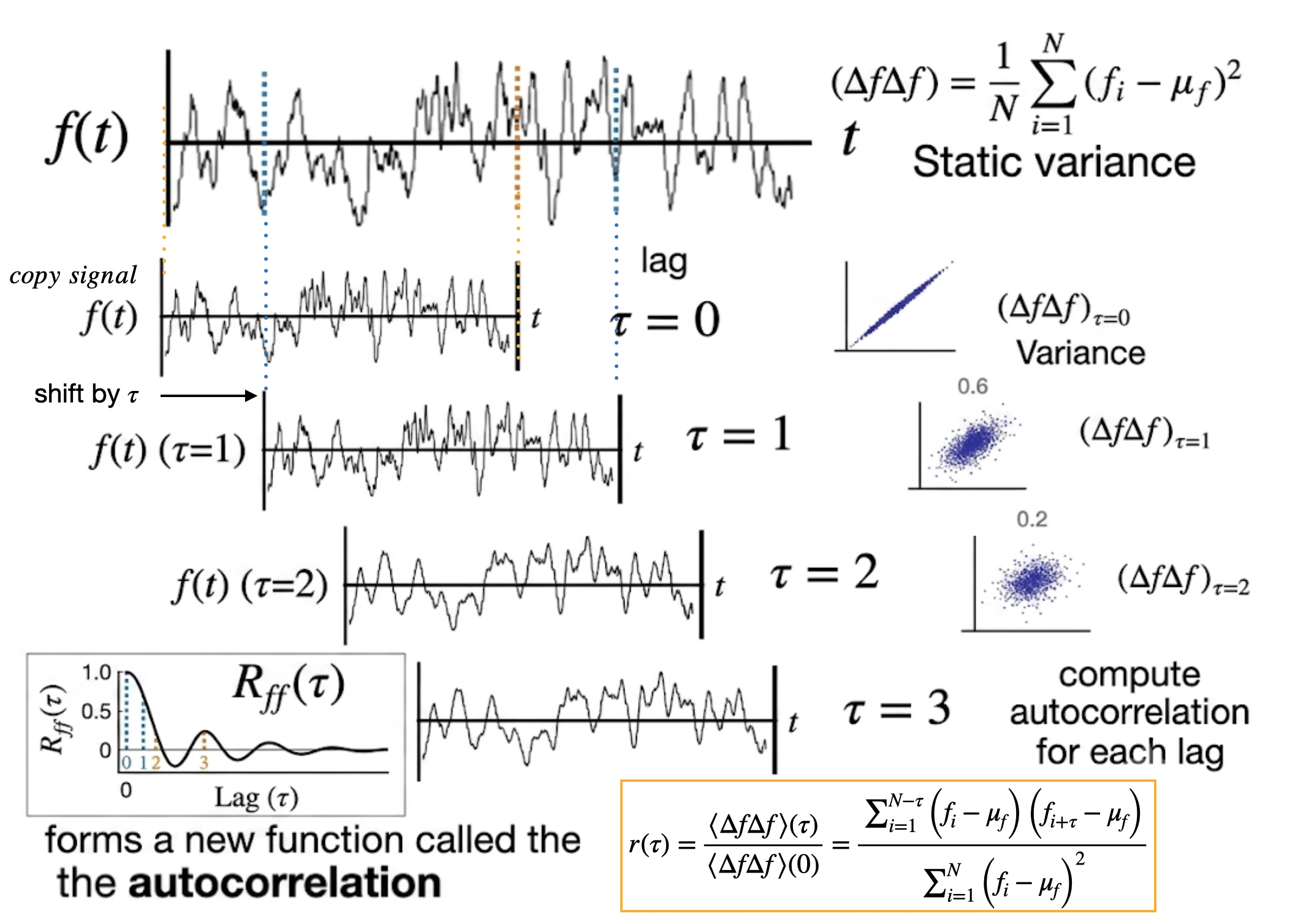
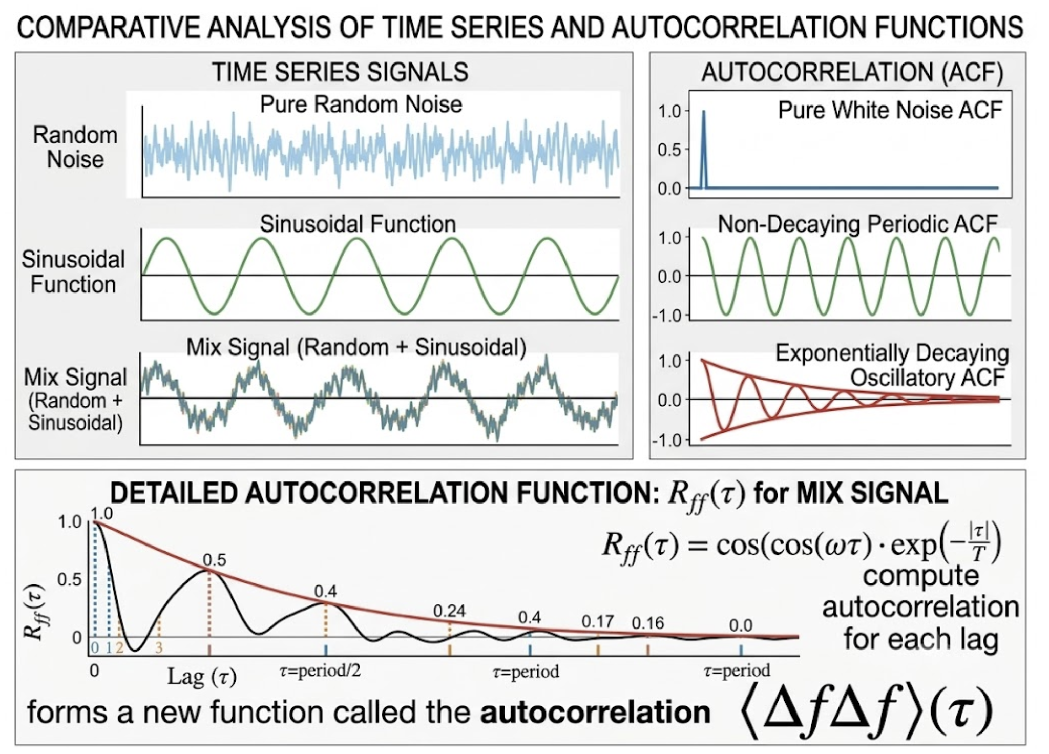
A magical idea: \(X \rightarrow X\) type learning
Yesterday's features can predict today's features 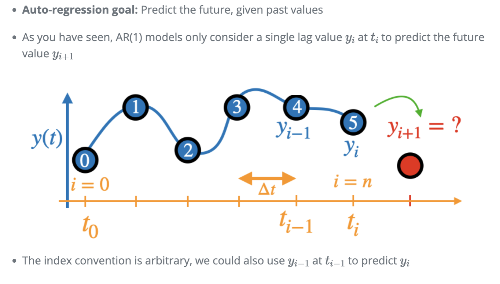
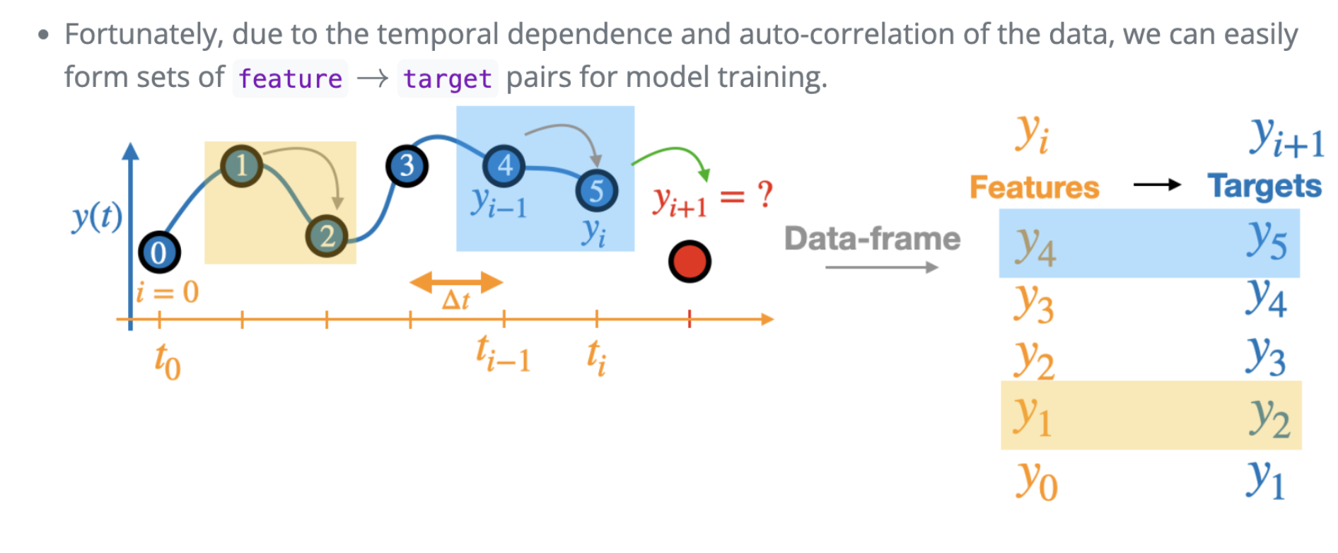
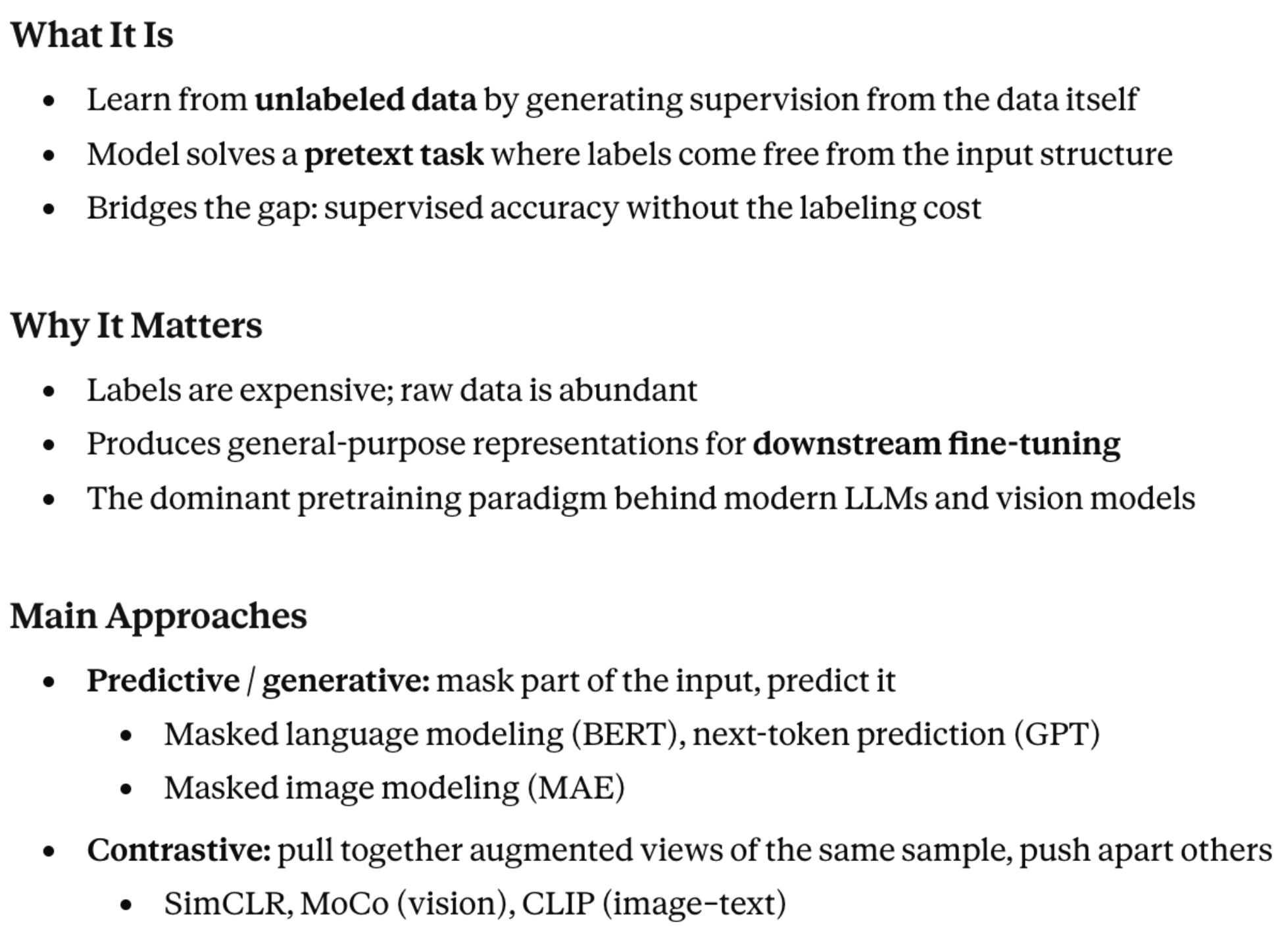
Self supervised learning s sort of fits between supervised and unsupervised learning because it doesn’t require an explicit human supervised
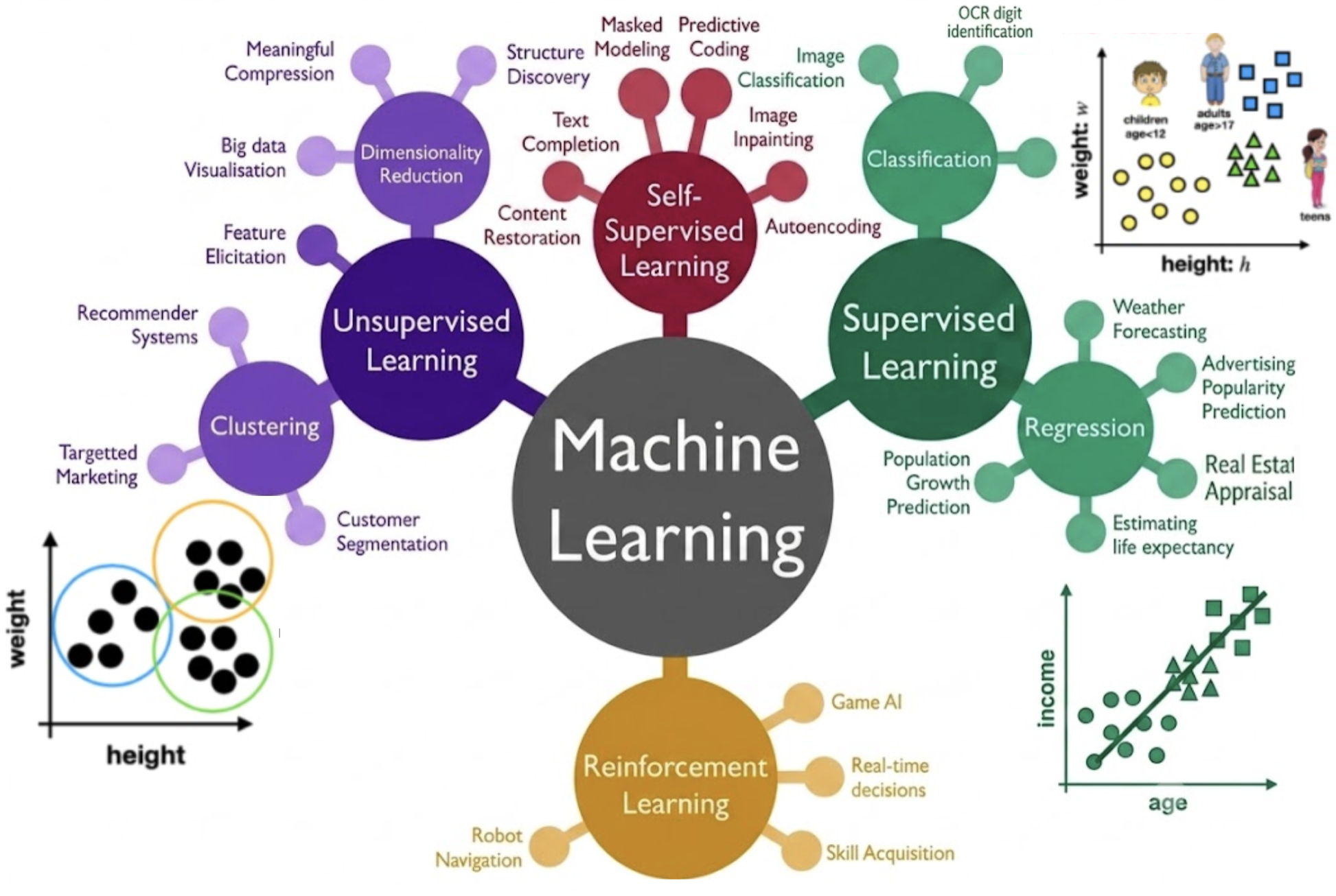
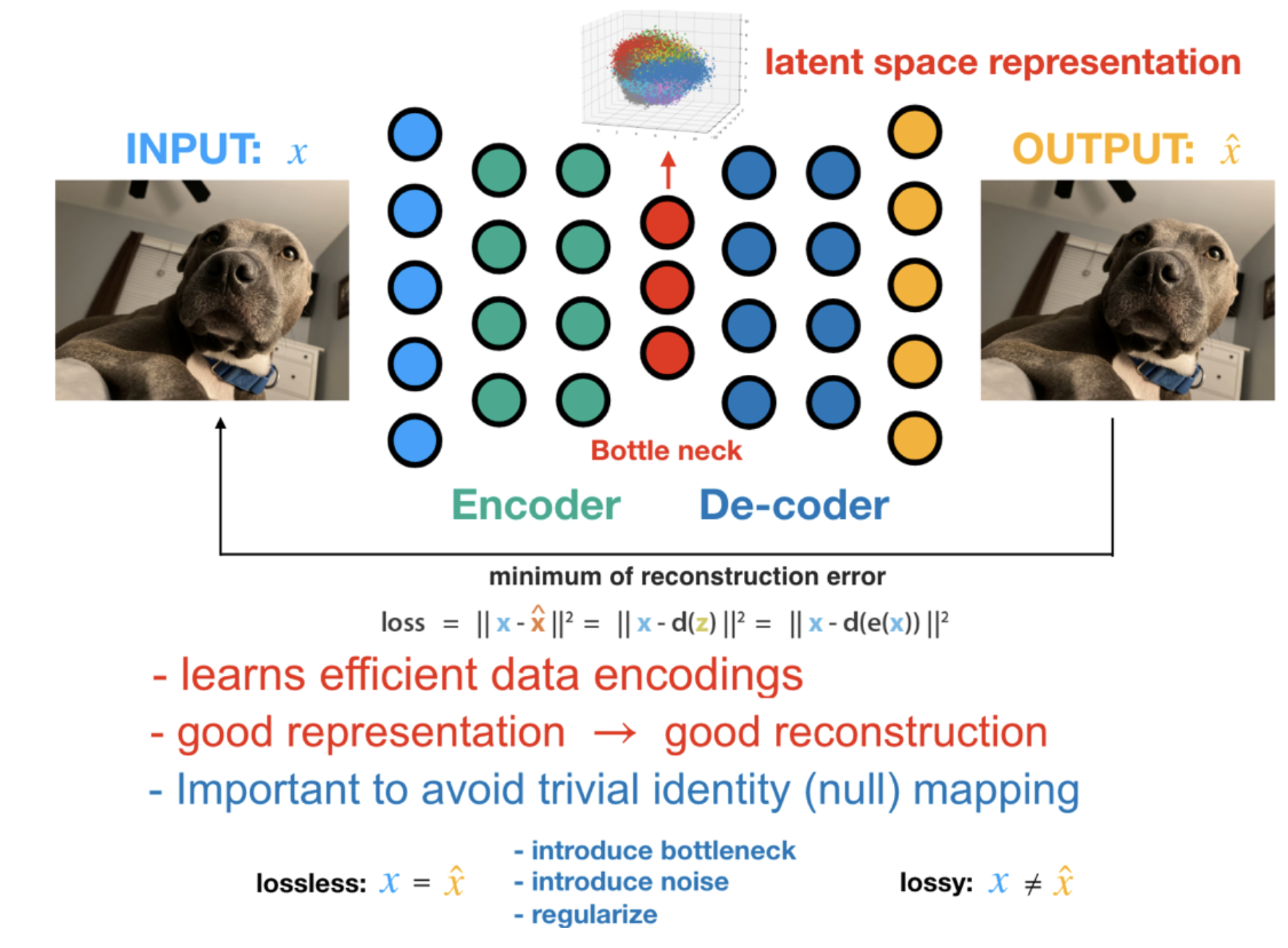
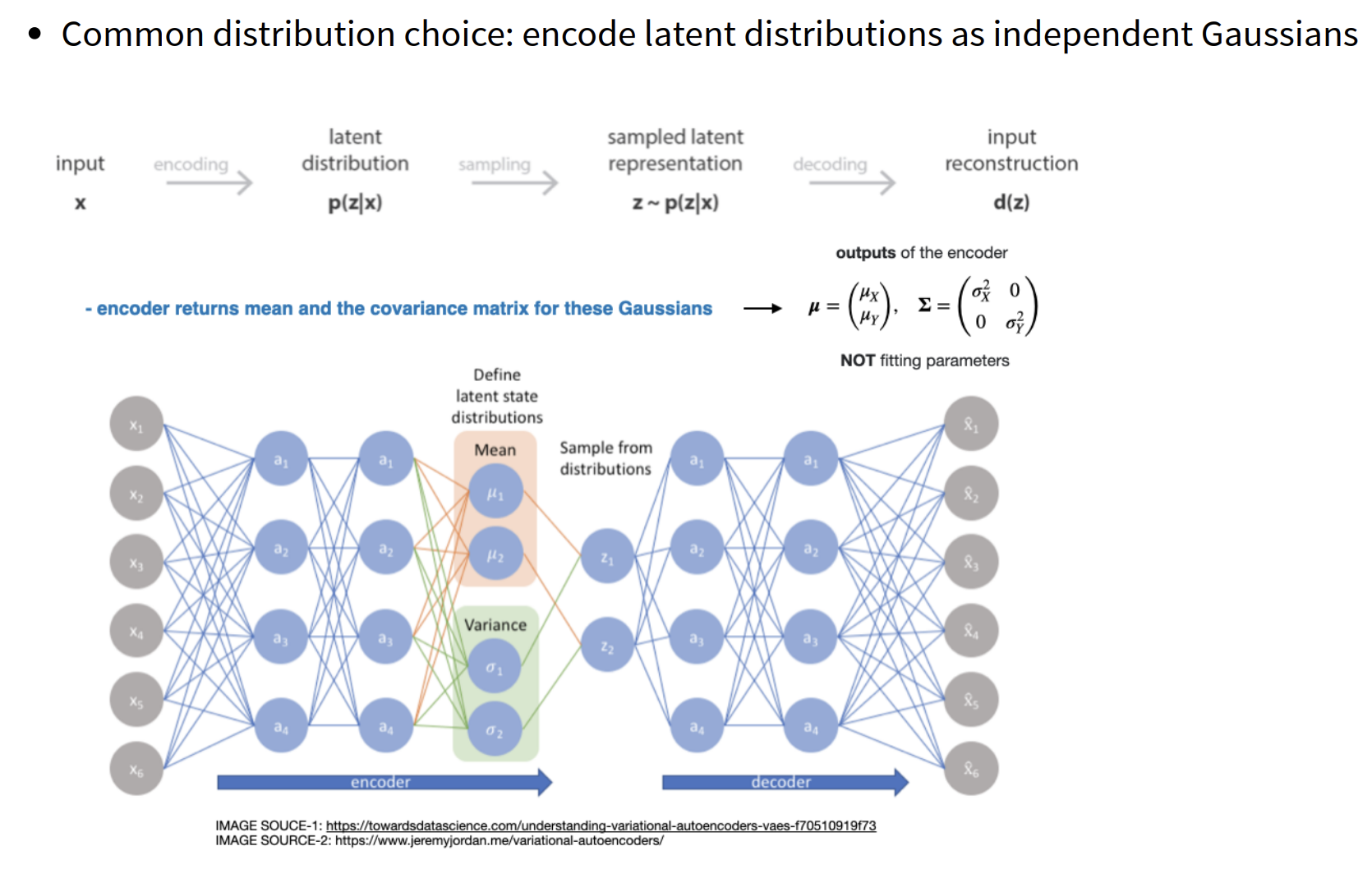
While not a time series model. The auto encoder is a textbook example of self supervision where the input and target pair X and Y come directly from the inputs themselves. There’s no need for human supervision.
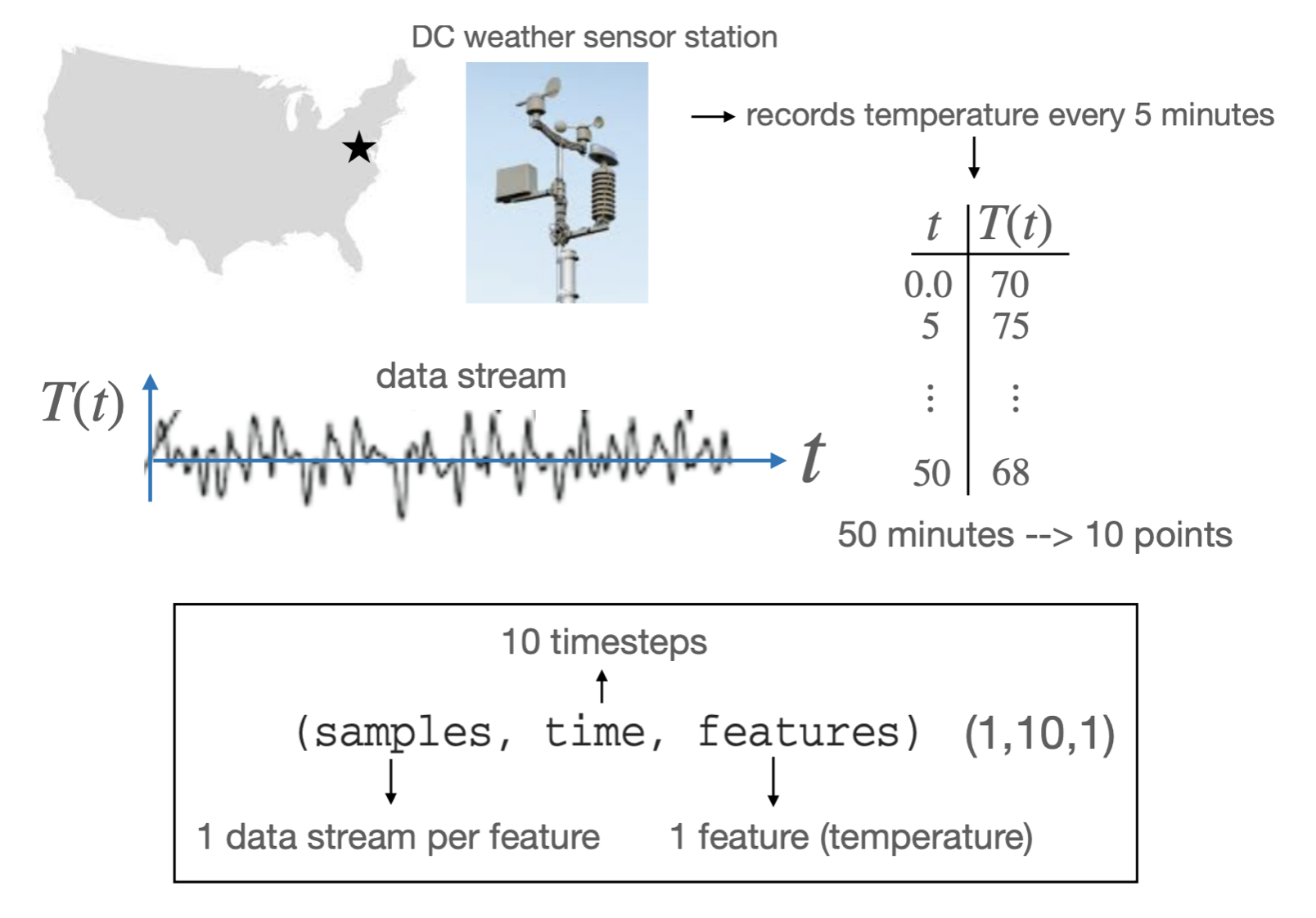
A univariate series is one number per timestep. Here: 12 days of (fake) temperature readings.
(12,): a flat vectortemp: [20 22 25 24 21 19 18 20 23 26 28 27]
shape: (12,)
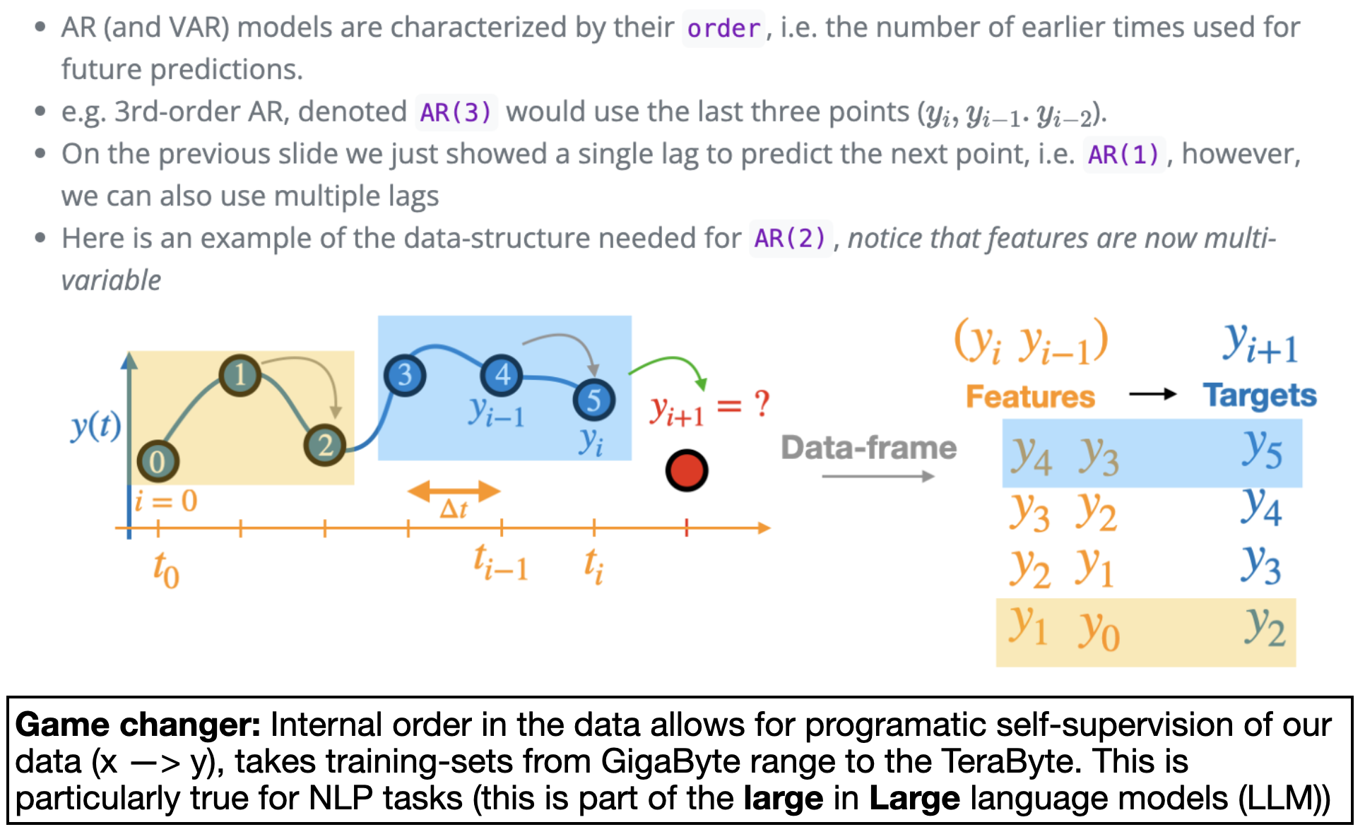
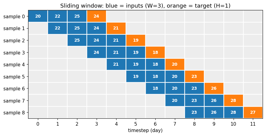
A model cannot learn from one long line. We cut it into many overlapping windows:
W: how many past timesteps the model sees (here W = 3)H: how far ahead we predict (here H = 1, the very next day)Slide the window forward one step at a time to generate every sample.
sample 0: X = [20 22 25]  ->  y = 24
sample 1: X = [22 25 24]  ->  y = 21
sample 2: X = [25 24 21]  ->  y = 19
sample 3: X = [24 21 19]  ->  y = 18
sample 4: X = [21 19 18]  ->  y = 20
sample 5: X = [19 18 20]  ->  y = 23
sample 6: X = [18 20 23]  ->  y = 26
sample 7: X = [20 23 26]  ->  y = 28
sample 8: X = [23 26 28]  ->  y = 27

X shape: (9, 3)  (samples, timesteps)
y shape: (9,)
Each row is one sample: blue cells are the window (inputs), orange is the target.
X_uni is (9, 3): but the model wants (samples, timesteps, features). A univariate series has exactly one feature, so we add a trailing axis of size 1.
(9, 3) → (9, 3, 1)before: (9, 3) -> after: (9, 3, 1)
sample 0 as a (timesteps, features) matrix:
[[20]
[22]
[25]]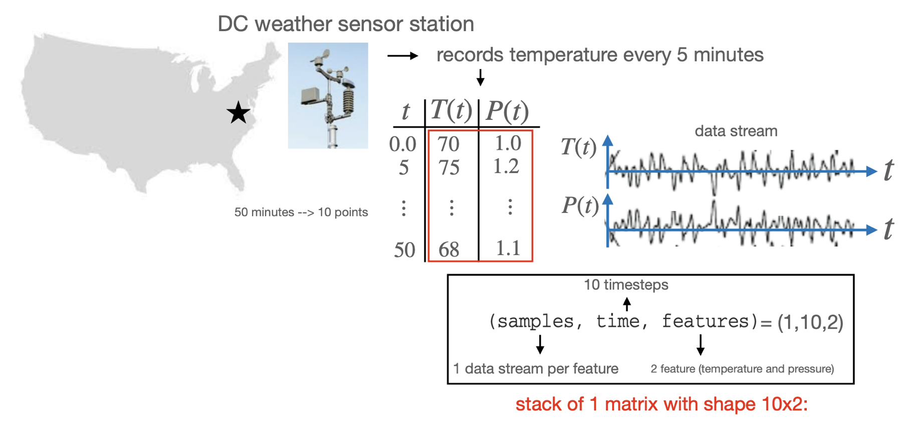
Now each timestep carries three measurements: temperature, humidity, wind.
(10, 3) = (timesteps, features)series shape: (10, 3) (timesteps, features)
[[20 65 5]
[22 60 7]
[25 55 6]
[24 58 4]
[21 70 9]
[19 75 12]
[18 80 11]
[20 72 8]
[23 64 6]
[26 58 5]]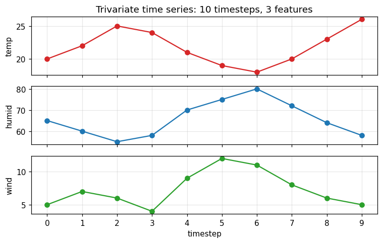
look-back three previous days
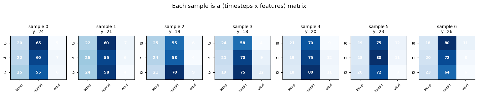
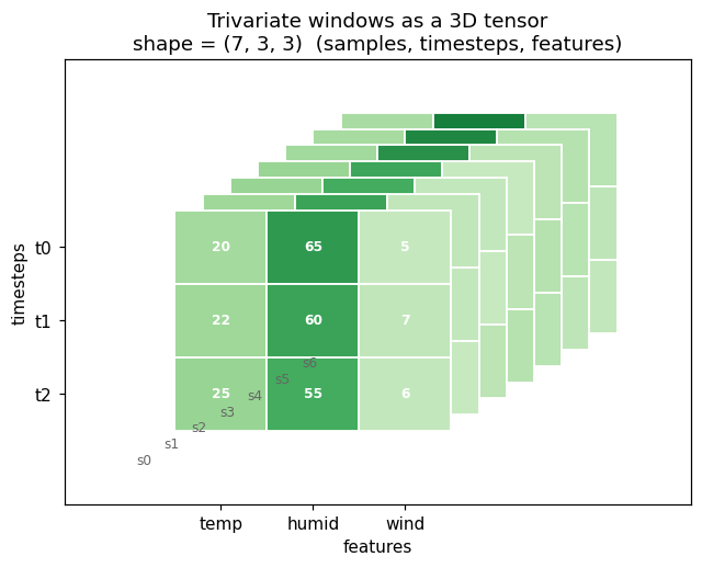
X shape: (7, 3, 3)  (samples, timesteps, features)
y shape: (7,)

sample 0 (rows = timesteps, cols = temp/humid/wind):
[[20 65  5]
 [22 60  7]
 [25 55  6]]

target 0: 24
Each sample is now a matrix, not a vector: 3 rows (time) by 3 columns (features). Stacking those matrices gives the 3D tensor.
Takeaway: the univariate and trivariate cases are the same code. Only the size of the last axis changes.
| case | raw data | one sample | tensor |
|---|---|---|---|
| univariate | (12,) |
(3, 1) |
(9, 3, 1) |
| trivariate | (10, 3) |
(3, 3) |
(7, 3, 3) |
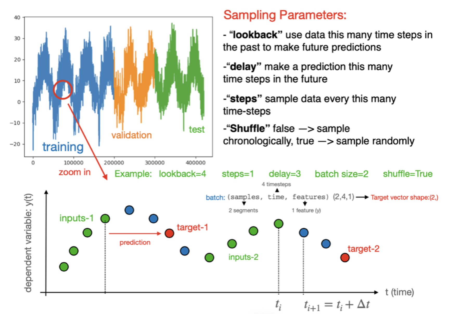
Standard k-fold cross-validation shuffles samples. That is invalid here:
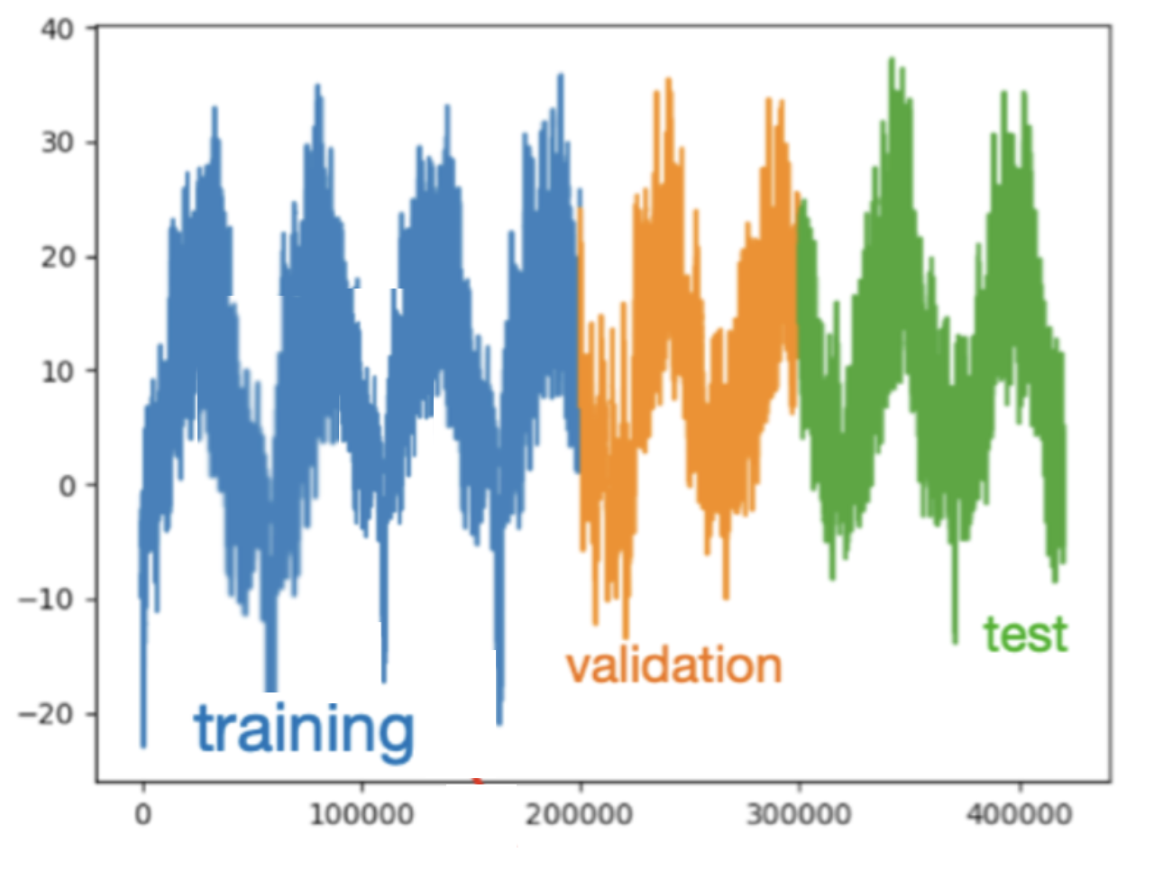
Note, similar to regular k-fold, we are training multiple models here. One per fold, and the aggregate scores a hyperparameter configuration rather than any individual model.
The simplest correct version is walk-forward (expanding window) validation:
fold 0: train = [np.int64(0), np.int64(1), np.int64(2), np.int64(3)]   val = [np.int64(4), np.int64(5)]
fold 1: train = [np.int64(0), np.int64(1), np.int64(2), np.int64(3), np.int64(4), np.int64(5)]   val = [np.int64(6), np.int64(7)]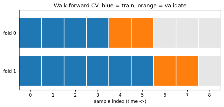
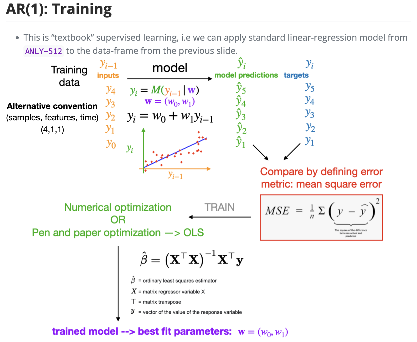
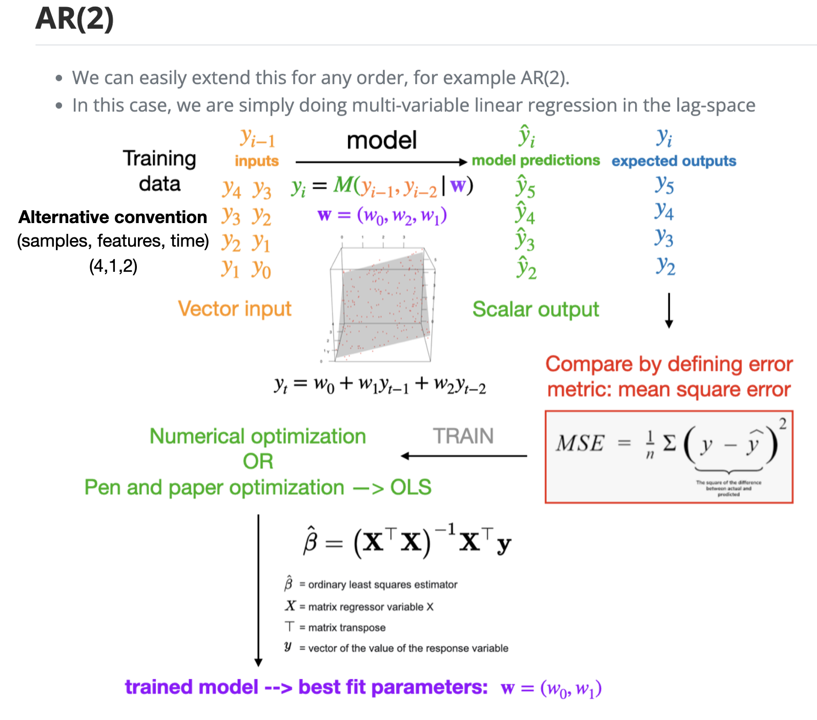
Note that we could also use a more complicated curve fitting model here, such as a multi-layer perceptron.
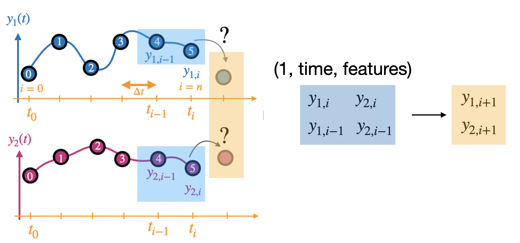
This that we flattened the vector here.
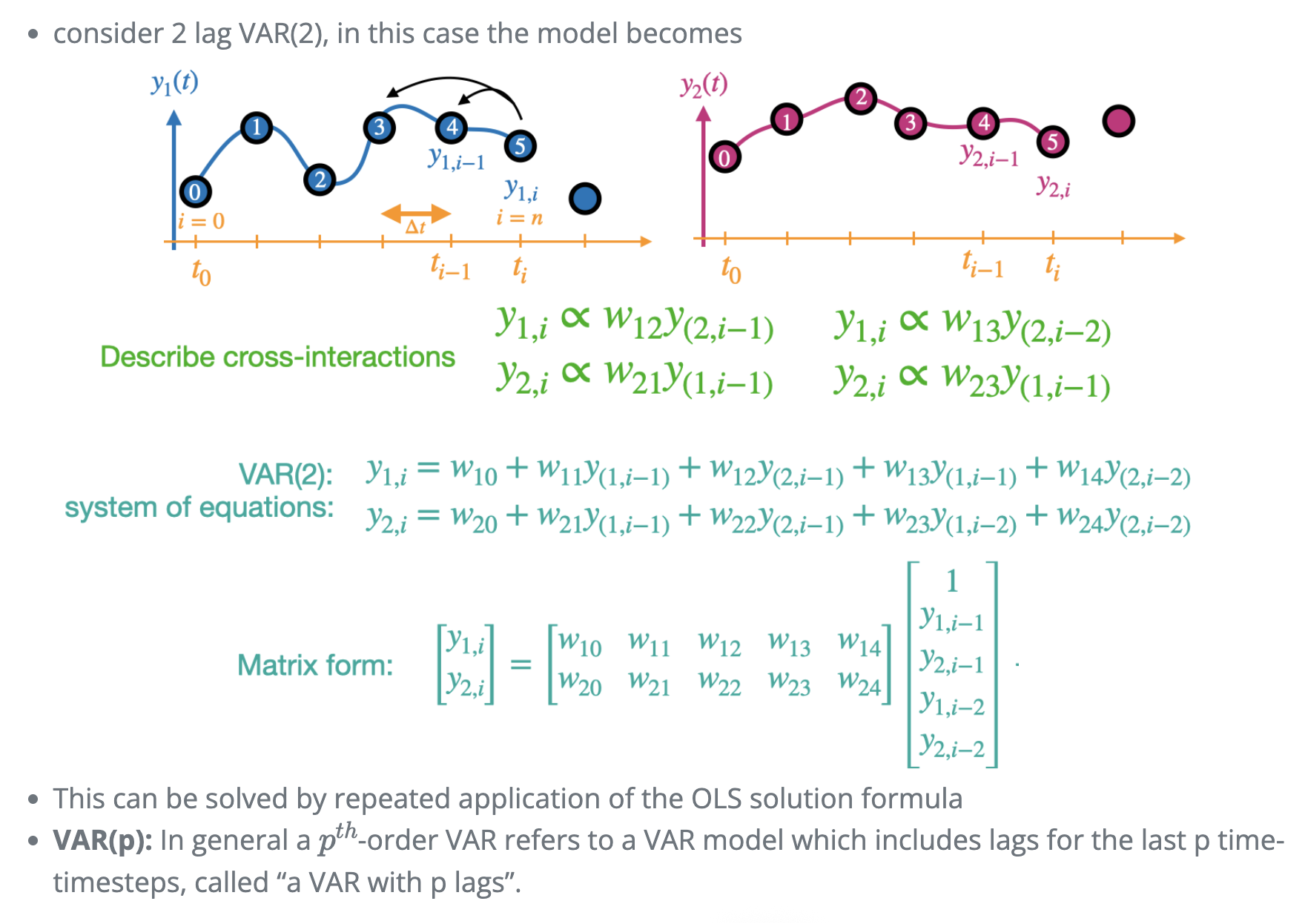
Text is also a sequence: timesteps are token positions instead of clock ticks. The target shape is identical:
(samples, timesteps, features)
    |          |          |
 sentences   words    word representation
The only new problem: a word is not a number. We need to invent the feature axis.
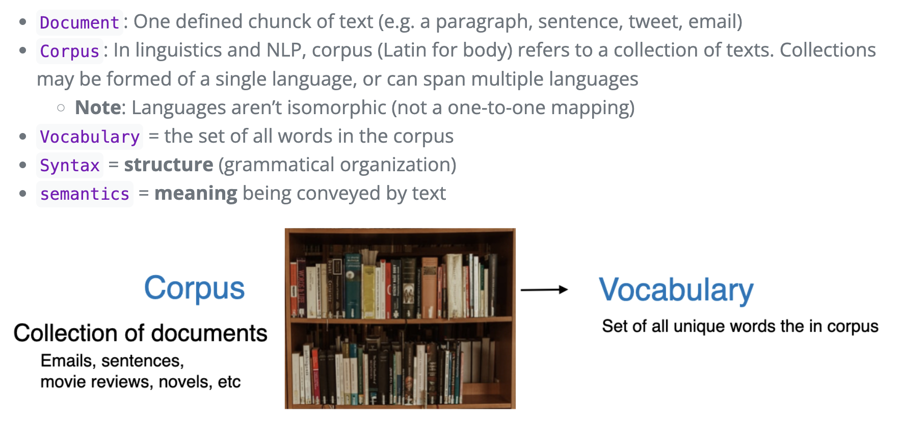
Two reserved ids come first by convention:
<pad> = 0: filler so all sequences have equal length<unk> = 1: any word not seen during trainingsentence 0: ['the', 'cat', 'sat', 'on', 'the', 'mat']
sentence 1: ['the', 'dog', 'sat', 'on', 'the', 'log']
sentence 2: ['a', 'cat', 'chased', 'the', 'dog']
sentence 3: ['the', 'dog', 'barked']
vocabulary size V = 12
{'<pad>': 0, '<unk>': 1, 'a': 2, 'barked': 3, 'cat': 4, 'chased': 5, 'dog': 6, 'log': 7, 'mat': 8, 'on': 9, 'sat': 10, 'the': 11}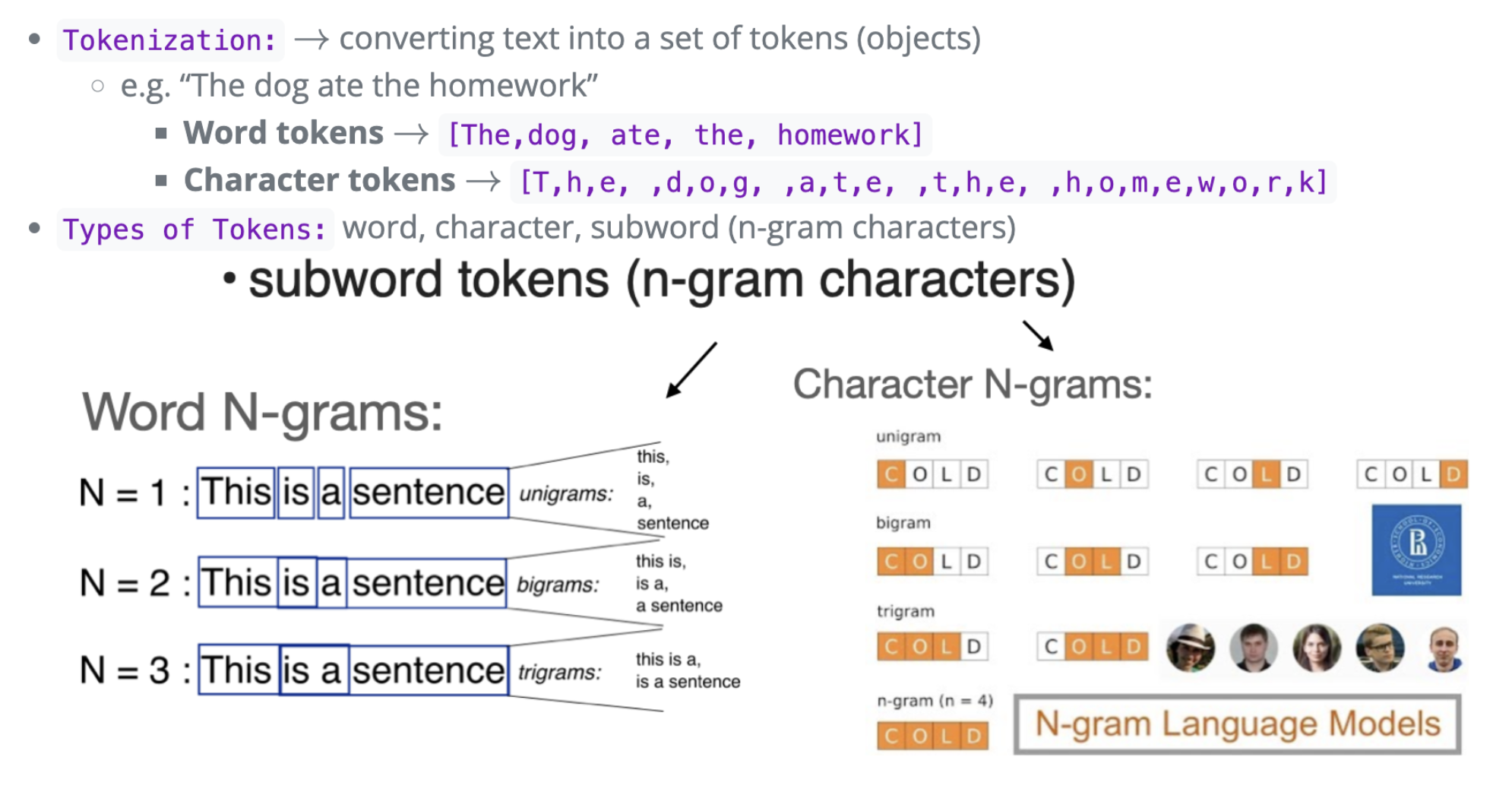

0 (and truncate long ones) to a fixed TResult is (samples, timesteps): integers, not yet features.
seqs shape: (4, 6)  (samples, timesteps)
[[11  4 10  9 11  8]
 [11  6 10  9 11  7]
 [ 2  4  5 11  6  0]
 [11  6  3  0  0  0]]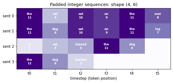
These integers are ids, not magnitudes. cat = 4 and dog = 6 does not mean a dog is 1.5 cats. Feeding raw ids to a model implies an ordering that does not exist, so we replace each id with a vector. Two ways to do that follow.
Shallow methods often simplify the vocabulary dramatically by truncating or simplifying words.
This is typically not done for deep models because they can handle the context, Do there increase model flexibility
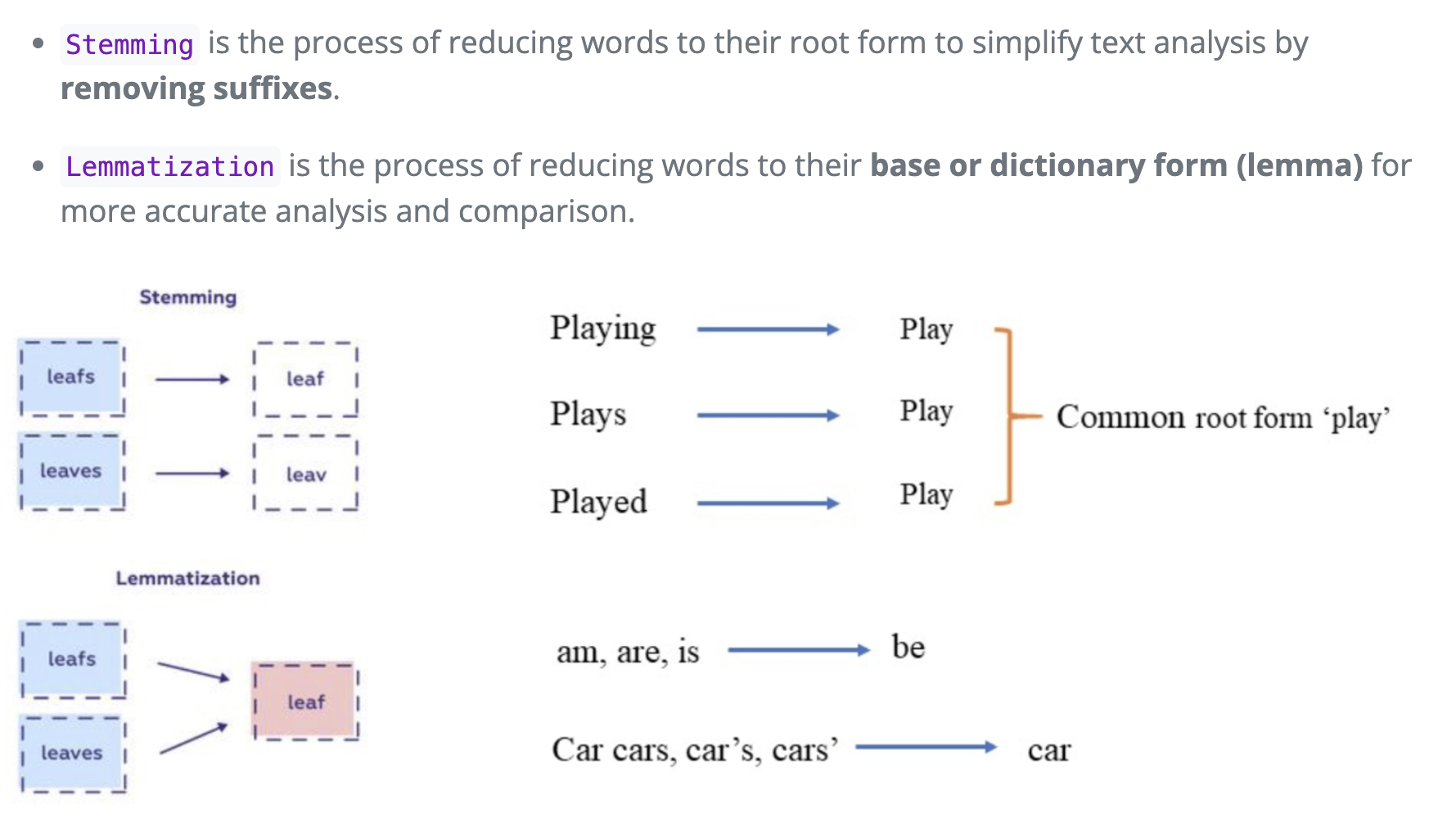
Classical NLP pipelines shrink the vocabulary by normalizing word forms before encoding:
running → run, studies → studi)better → good, ran → run)Why it used to matter:
V means smaller one-hot vectors and fewer embedding rowsrun / running / ran each get too few examples to learn from separately word | stem | lemma
running | run | run
runs | run | run
ran | ran | run
studies | studi | study
cats | cat | cats
barked | bark | barked
better | better | goodBag of words (BoW) counts the words in a sentence and forgets where they were.
(samples, timesteps, V) to (samples, V): rank 2, no time axisThe classic failure case: two sentences with opposite meanings produce the identical BoW vector.
Modern practice mostly drops these steps. Contemporary models rarely stem or lemmatize because:
running into pieces like run + ##ning, so related forms share representation without any hand-written rulesrun, ran, and running are related, and they place those embeddings near each otherstudies → studi), and tense/number/aspect often matter for the taskV with a single 1 in its own slot(samples, timesteps, V): the feature axis is the whole vocabularyProperties:
Vonehot shape: (4, 6, 12) (samples, timesteps, features=V)
sentence 0, timestep 1 -> cat
[0 0 0 0 1 0 0 0 0 0 0 0]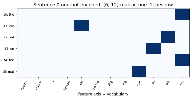
nonzeros: 6 out of 72 cells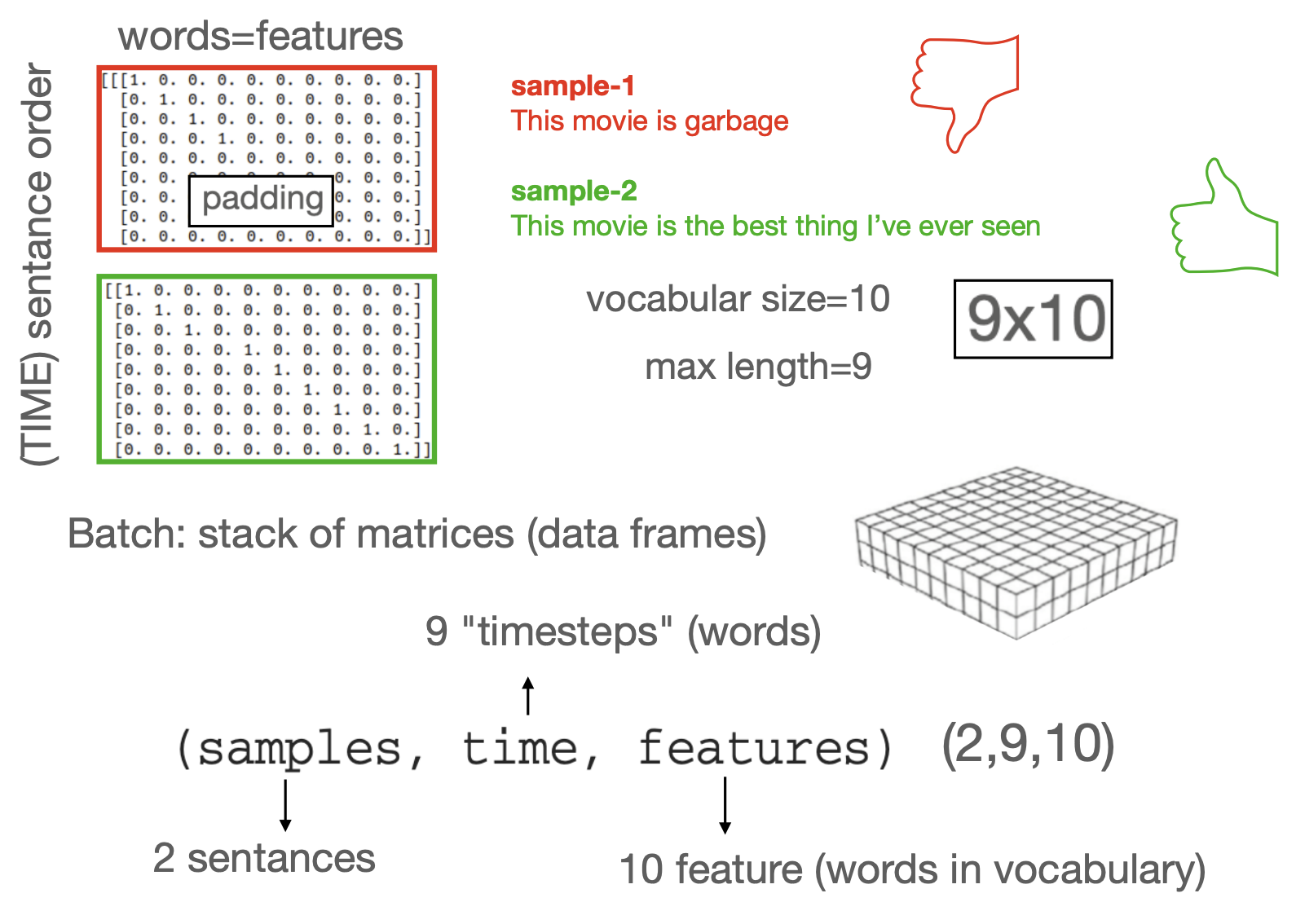
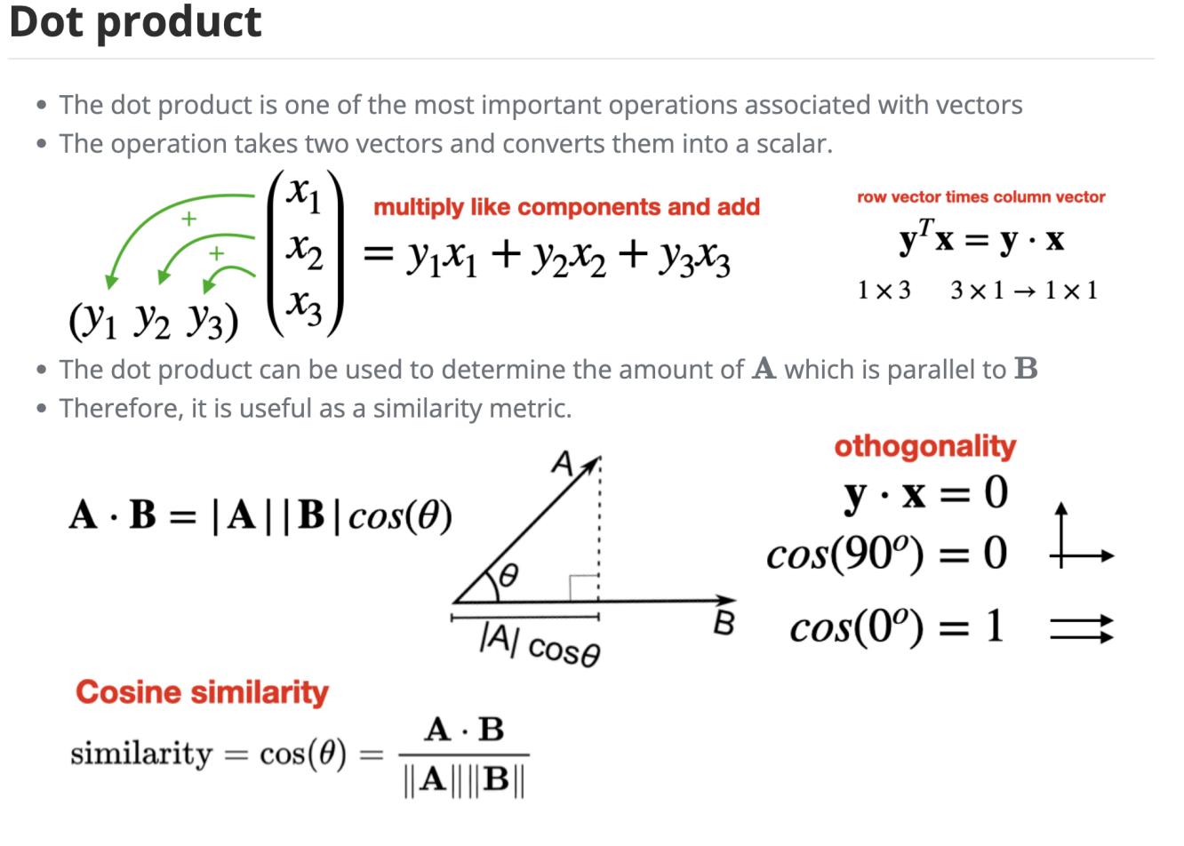
Cosine similarity between any two different one-hot words is exactly 0: “cat” is as unrelated to “dog” as it is to “on”.
cos(cat, dog) = 0.0
cos(cat, on ) = 0.0
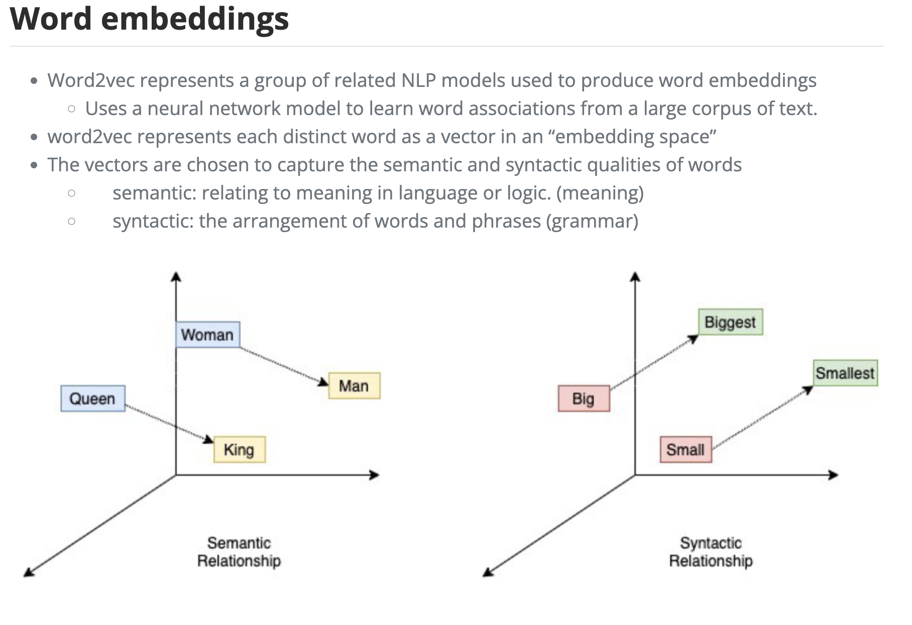
cos(cat, cat) = 1.0Replace the length-V sparse vector with a short dense vector of length d (d << V).
E has shape (V, d): one row per vocabulary wordE[seqs] → (samples, timesteps, d)Below d = 2 and the vectors are handcrafted so the geometry is visible. Real models use d in the 100s and learn E by gradient descent.
E shape: (12, 2) (vocab, embedding_dim)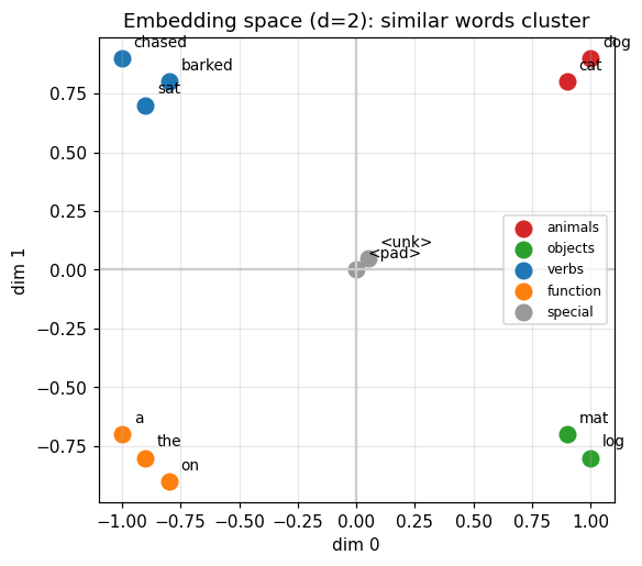
embedded shape: (4, 6, 2)  (samples, timesteps, features=d)

sentence 0:
  t0     the  ->  [-0.9 -0.8]
  t1     cat  ->  [0.9 0.8]
  t2     sat  ->  [-0.9  0.7]
  t3      on  ->  [-0.8 -0.9]
  t4     the  ->  [-0.9 -0.8]
  t5     mat  ->  [ 0.9 -0.7]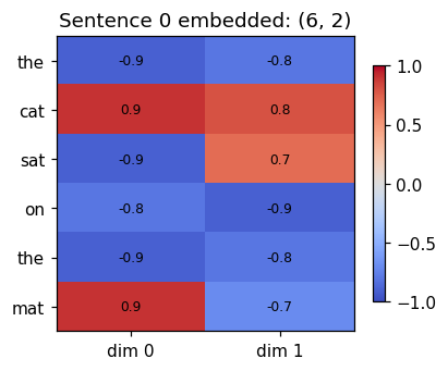
One-hot and embedding are the same operation. A one-hot row times E selects a row of E, so an embedding layer is a matrix multiply that we implement as a lookup for speed.
onehot @ E == E[seqs]
identical: True

feature-axis size: one-hot = 12 vs dense = 2| representation | shape | time axis? | notes |
|---|---|---|---|
| raw univariate series | (12,) |
implicit | one long sequence |
| windowed univariate | (9, 3, 1) |
yes | feature axis added by hand |
| raw trivariate series | (10, 3) |
implicit | features in last column |
| windowed trivariate | (7, 3, 3) |
yes | each sample is a matrix |
| integer sequences | (4, 6) |
yes | ids only, not usable features |
| one-hot text | (4, 6, 12) |
yes | sparse, no similarity |
| embedded text | (4, 6, 2) |
yes | dense, learned, similarity-aware |
| bag of words | (4, 12) |
no | order destroyed |
The recurring recipe:
X.shape before it reaches the model