LSTM
Recording
LSTM big picture overview
This recording provides a big picture overview of the LSTM architecture.
Feel free to watch at 1.5x or 2x speed.
Note: If you find something missing or incorrect in the recording, then please let me know!
LSTM sample calculation
This recording demonstrates a sample evaluation of an LSTM for a given input sentence.
This is the core focus of the lecture, there are some additional details in the notes below which are not covered in the recording, which are are encouraged to review at your own pace.
Feel free to watch at 1.5x or 2x speed.
Note: If you find something missing or incorrect in the recording, then please let me know!
Long Short-Term Memory (LSTM) Networks
Motivation
- LSTMs are a advanced version of RNNs that are able to learn long-term dependencies.
- They are able to capture complex patterns in time series data.
- They also help mitigate the problem of vanishing and exploding gradients by using a gating mechanism, which allows the model to selectively remember or forget information.
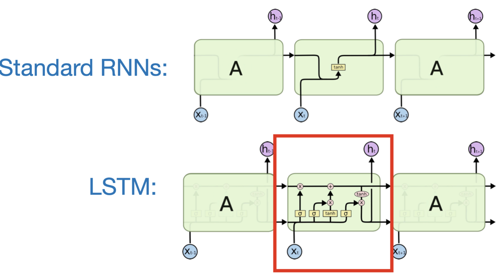
Recall: Simple RNN
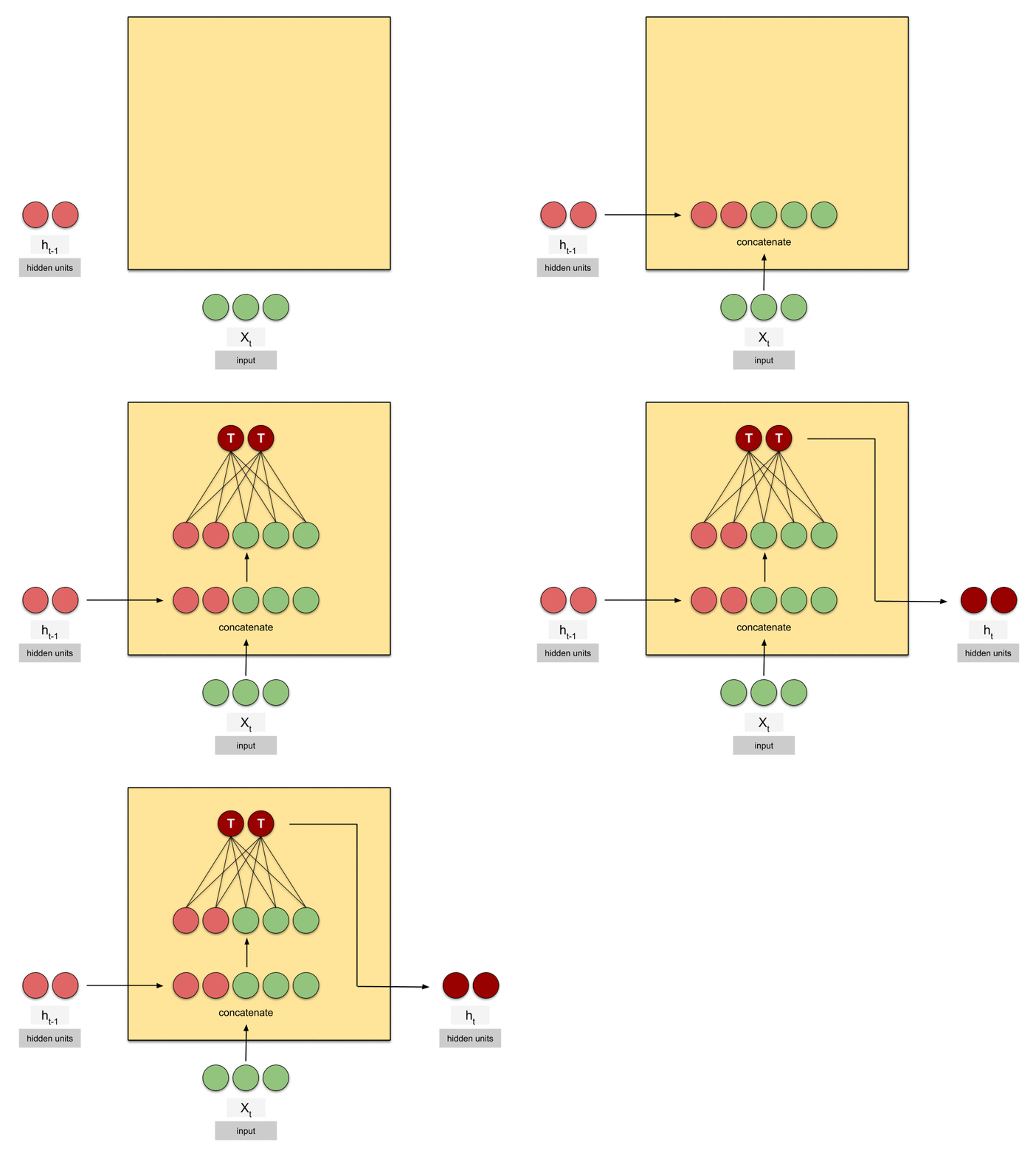
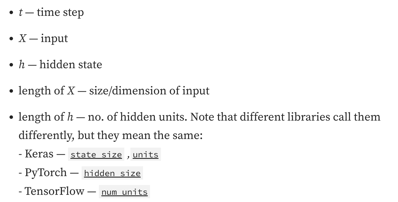
Source: https://medium.com/data-science/animated-rnn-lstm-and-gru-ef124d06cf45
Recall: Vanishing and Exploding Gradients
- Vanishing gradients: Gradients become too small for effective learning.
- Exploding gradients: Gradients become excessively large, destabilizing learning.
Both hinder learning long-term dependencies.
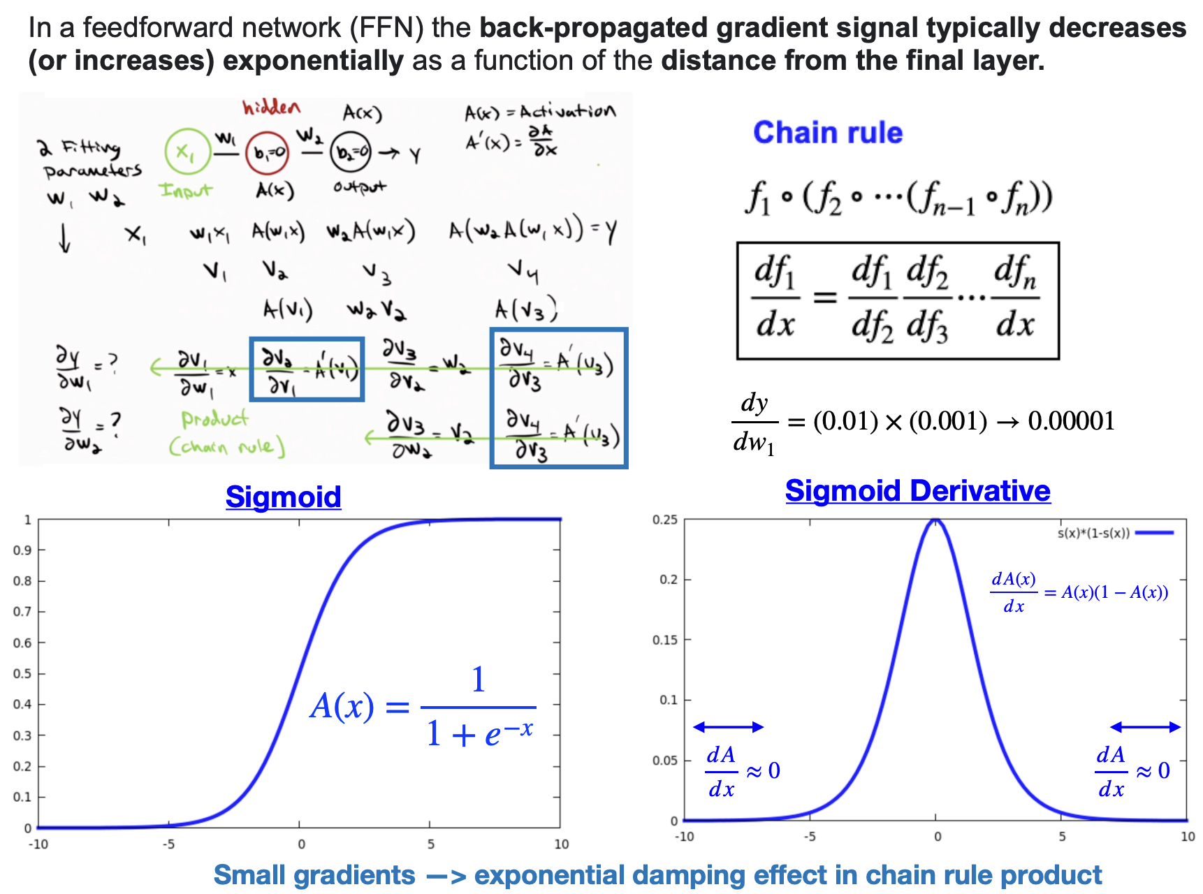
Backpropagation Through Time (BPTT)
- Idea: Train an RNN by applying backpropagation to its time-unrolled computational graph.
- Unroll the RNN over time steps \(t=1 \ldots T\).
- Forward pass: compute hidden states/outputs in sequence.
- Compute total loss over all time steps.
- Backward pass: propagate gradients backward through time to update shared weights.
- Key: the same parameters are reused at each time step, so gradients are summed across time.
- Challenge: long sequences may cause vanishing or exploding gradients. For example, for shared weight \(W\) and loss over \(T\) steps, the total gradient sums contributions from each step:
\[ \frac{\partial L}{\partial W}=\sum_{t=1}^T \frac{\partial L_t}{\partial W} \]
So when slides say “gradients accumulate across time”, they mean: - each time step produces a gradient contribution - these contributions are summed before updating the parameter.
Vanishing Gradients
- Vanishing gradients are a major limitation of simple RNNs.
- As a result, the impact of early time steps is lost over time.
- Simple RNNs typically exhibit only short-term memory, able to retrieve information from only the previous 10 to 100 inputs.
- As a result, simple RNNs are too simplistic and are rarely used in practice.
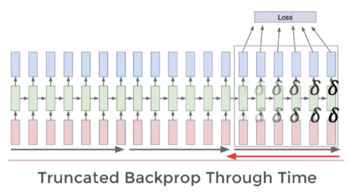
Mitigating the effect
- this is often mitigated by truncation, gradient clipping
- Or by using gated RNNs like LSTM or GRU (introduced by Hochreiter and Schmidhuber in 1997).
LSTM Example Calculation
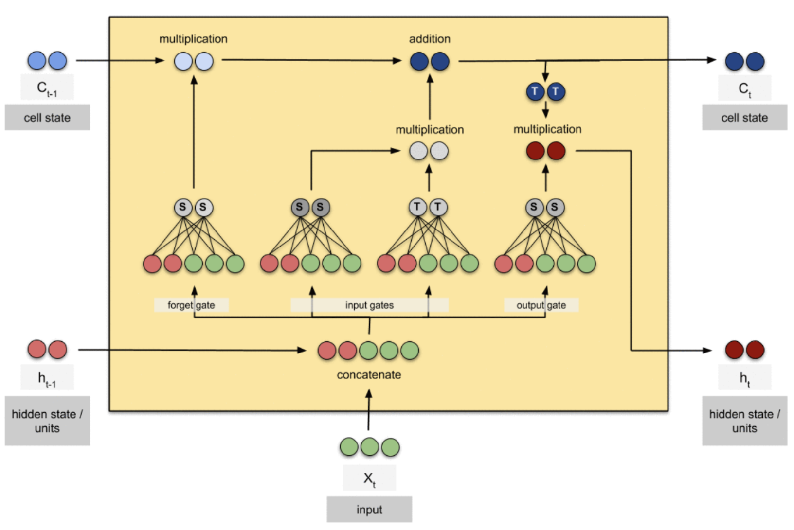
Example: Tiny LSTM evaluation
Consider the sentence: I eat bread with the following design choices
- input dimension = 3
- hidden state dimension = 2
- cell state dimension = 2
- 3 time steps:
I,eat,bread
\[ h_0 = \begin{bmatrix}0\\0\end{bmatrix}, \qquad c_0 = \begin{bmatrix}0\\0\end{bmatrix} \]
Image Source: https://medium.com/data-science/animated-rnn-lstm-and-gru-ef124d06cf45
Vocabulary and one-hot inputs
Vocabulary:
I\(\to [1,0,0]^T\)eat\(\to [0,1,0]^T\)bread\(\to [0,0,1]^T\)
So:
\[ x_1 = \begin{bmatrix}1\\0\\0\end{bmatrix}, \quad x_2 = \begin{bmatrix}0\\1\\0\end{bmatrix}, \quad x_3 = \begin{bmatrix}0\\0\\1\end{bmatrix} \]
LSTM equations
At time step \(t\):
\[ \begin{gathered} f_t=\sigma\left(W_f x_t+U_f h_{t-1}+b_f\right) \\ i_t=\sigma\left(W_i x_t+U_i h_{t-1}+b_i\right) \\ \tilde{c}_t=\tanh \left(W_c x_t+U_c h_{t-1}+b_c\right) \\ o_t=\sigma\left(W_o x_t+U_o h_{t-1}+b_o\right) \\ c_t=f_t \odot c_{t-1}+i_t \odot \tilde{c}_t \\ h_t=o_t \odot \tanh \left(c_t\right) \end{gathered} \]
Fitting Parameter matrices
Forget gate
\[ W_f = \begin{bmatrix} 1 & 0 & 0 \\ 0 & 1 & 1 \end{bmatrix}, \qquad U_f = \begin{bmatrix} 1 & 0 \\ 0 & 1 \end{bmatrix}, \qquad b_f = \begin{bmatrix} 0\\1 \end{bmatrix} \]
Input gate
\[ W_i = \begin{bmatrix} 1 & 1 & 0 \\ 0 & 1 & 1 \end{bmatrix}, \qquad U_i = \begin{bmatrix} 1 & 0 \\ 1 & 1 \end{bmatrix}, \qquad b_i = \begin{bmatrix} 1\\0 \end{bmatrix} \]
Candidate cell update
\[ W_c = \begin{bmatrix} 1 & 0 & 1 \\ 0 & 1 & 1 \end{bmatrix}, \qquad U_c = \begin{bmatrix} 1 & 0 \\ 0 & 1 \end{bmatrix}, \qquad b_c = \begin{bmatrix} 0\\1 \end{bmatrix} \]
Output gate
\[ W_o = \begin{bmatrix} 1 & 0 & 1 \\ 1 & 1 & 0 \end{bmatrix}, \qquad U_o = \begin{bmatrix} 1 & 1 \\ 0 & 1 \end{bmatrix}, \qquad b_o = \begin{bmatrix} 0\\1 \end{bmatrix} \]
Useful approximations
We will use: \[ \sigma(0)=0.500,\quad \sigma(1)=0.731,\quad \sigma(2)=0.881 \] and \[ \tanh(0)=0,\quad \tanh(1)=0.762,\quad \tanh(2)=0.964 \] Also: \[ \tanh(0.670)\approx 0.585,\qquad \tanh(1.432)\approx 0.892 \]
Input and history concatenation
Recall there are two mathematical equivalent ways to compute:
- Do two separate matrix multiplications
- Combine (concatenate) the history and new input and evaluate with a single matrix operation
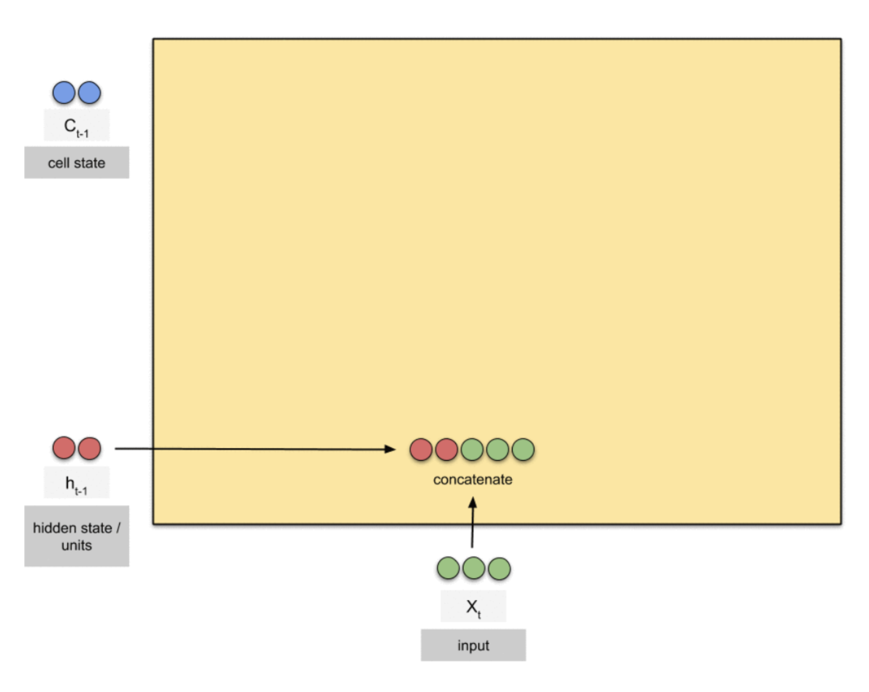
Processing Word-1: “I”
Step 1: process the word I
\[ x_1 = \begin{bmatrix}1\\0\\0\end{bmatrix} \]
Historical information (initialized to zero at time-step zero) \[ h_0 = \begin{bmatrix}0\\0\end{bmatrix}, \qquad c_0 = \begin{bmatrix}0\\0\end{bmatrix} \]
Forget gate calculation
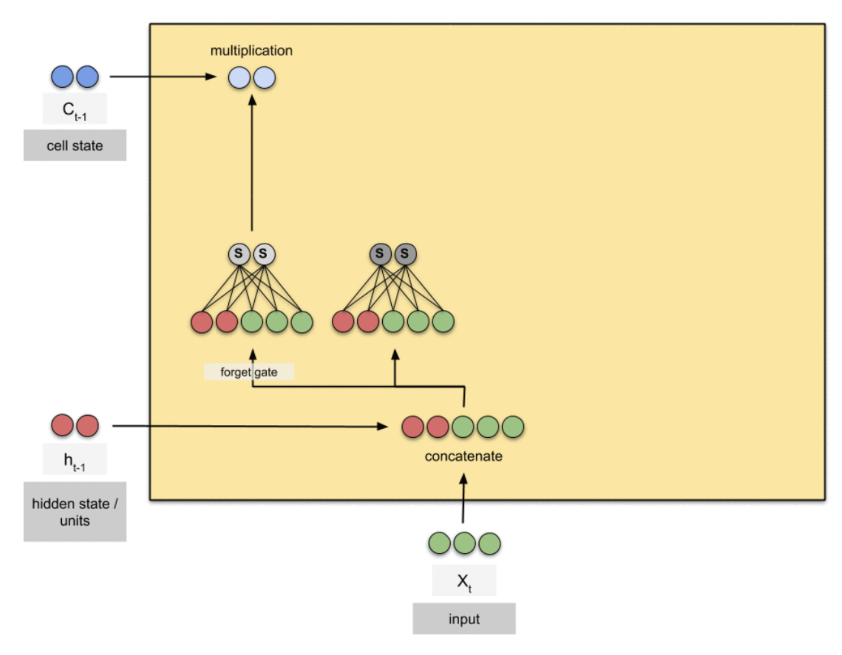
Forget gate decides how much of the previous cell memory to keep or erase.
\[ f_t=\sigma\left(W_f x_t+U_f h_{t-1}+b_f\right) \\ \]
\[ W_f = \begin{bmatrix} 1 & 0 & 0 \\ 0 & 1 & 1 \end{bmatrix}, \qquad U_f = \begin{bmatrix} 1 & 0 \\ 0 & 1 \end{bmatrix}, \qquad b_f = \begin{bmatrix} 0\\1 \end{bmatrix} \]
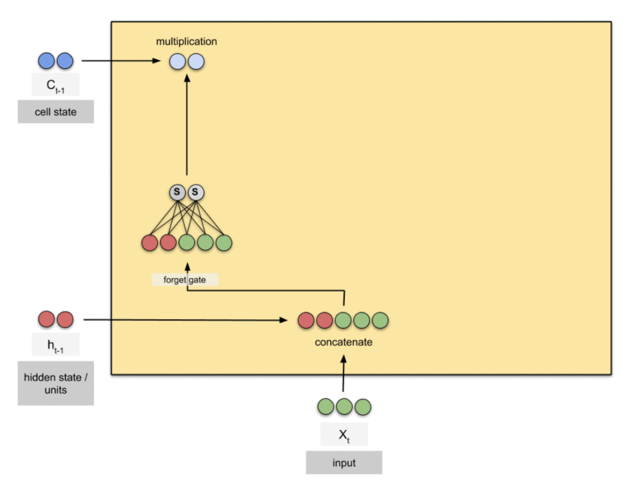
First compute: \[ W_f x_1 = \begin{bmatrix} 1 & 0 & 0 \\ 0 & 1 & 1 \end{bmatrix} \begin{bmatrix}1\\0\\0\end{bmatrix} = \begin{bmatrix}1\\0\end{bmatrix} \] So: \[ W_f x_1 + U_f h_0 + b_f = \begin{bmatrix}1\\0\end{bmatrix} + \begin{bmatrix}0\\0\end{bmatrix} + \begin{bmatrix}0\\1\end{bmatrix} = \begin{bmatrix}1\\1\end{bmatrix} \] Thus: \[ f_1 = \sigma\left(\begin{bmatrix}1\\1\end{bmatrix}\right) = \begin{bmatrix}0.731\\0.731\end{bmatrix} \]
Input gate calculation: part-1
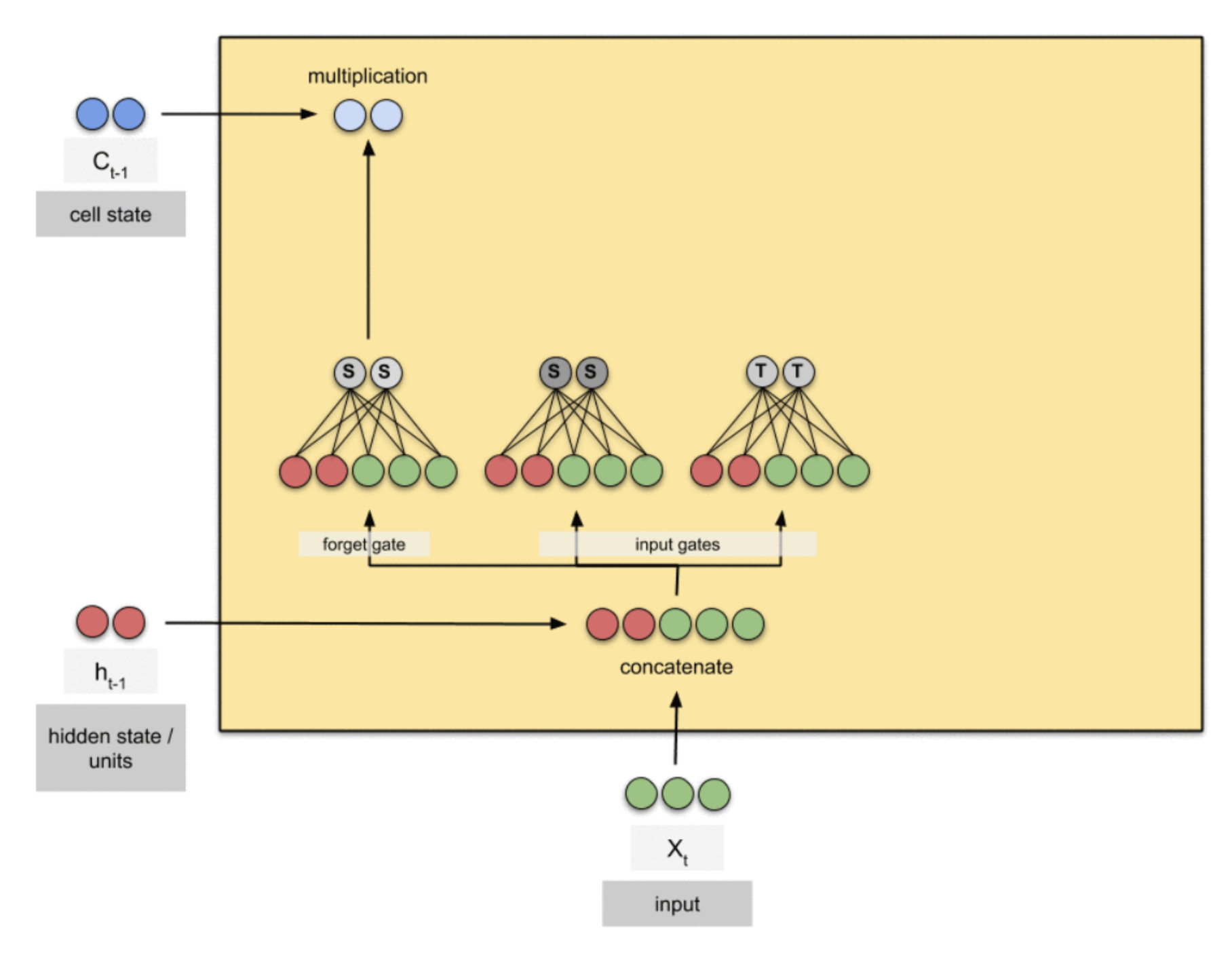
Input gate decides how much new information should be written into the cell state.
\[ i_t=\sigma\left(W_i x_t+U_i h_{t-1}+b_i\right) \\ \]
\[ W_i = \begin{bmatrix} 1 & 1 & 0 \\ 0 & 1 & 1 \end{bmatrix}, \qquad U_i = \begin{bmatrix} 1 & 0 \\ 1 & 1 \end{bmatrix}, \qquad b_i = \begin{bmatrix} 1\\0 \end{bmatrix} \]
\[ W_i x_1 = \begin{bmatrix} 1 & 1 & 0 \\ 0 & 1 & 1 \end{bmatrix} \begin{bmatrix}1\\0\\0\end{bmatrix} = \begin{bmatrix}1\\0\end{bmatrix} \]
So: \[ W_i x_1 + U_i h_0 + b_i = \begin{bmatrix}1\\0\end{bmatrix} + \begin{bmatrix}0\\0\end{bmatrix} + \begin{bmatrix}1\\0\end{bmatrix} = \begin{bmatrix}2\\0\end{bmatrix} \] Hence: \[ i_1 = \sigma\left(\begin{bmatrix}2\\0\end{bmatrix}\right) = \begin{bmatrix}0.881\\0.500\end{bmatrix} \]
Candidate cell state
Candidate state proposes the new content that could be added to the cell memory.
\[ \tilde{c}_t=\tanh \left(W_c x_t+U_c h_{t-1}+b_c\right) \\ \]
\[ W_c = \begin{bmatrix} 1 & 0 & 1 \\ 0 & 1 & 1 \end{bmatrix}, \qquad U_c = \begin{bmatrix} 1 & 0 \\ 0 & 1 \end{bmatrix}, \qquad b_c = \begin{bmatrix} 0\\1 \end{bmatrix} \]
\[ W_c x_1 = \begin{bmatrix} 1 & 0 & 1 \\ 0 & 1 & 1 \end{bmatrix} \begin{bmatrix}1\\0\\0\end{bmatrix} = \begin{bmatrix}1\\0\end{bmatrix} \]
So: \[ W_c x_1 + U_c h_0 + b_c = \begin{bmatrix}1\\0\end{bmatrix} + \begin{bmatrix}0\\0\end{bmatrix} + \begin{bmatrix}0\\1\end{bmatrix} = \begin{bmatrix}1\\1\end{bmatrix} \] Thus: \[ \tilde{c}_1 = \tanh\left(\begin{bmatrix}1\\1\end{bmatrix}\right) = \begin{bmatrix}0.762\\0.762\end{bmatrix} \]
Cell update
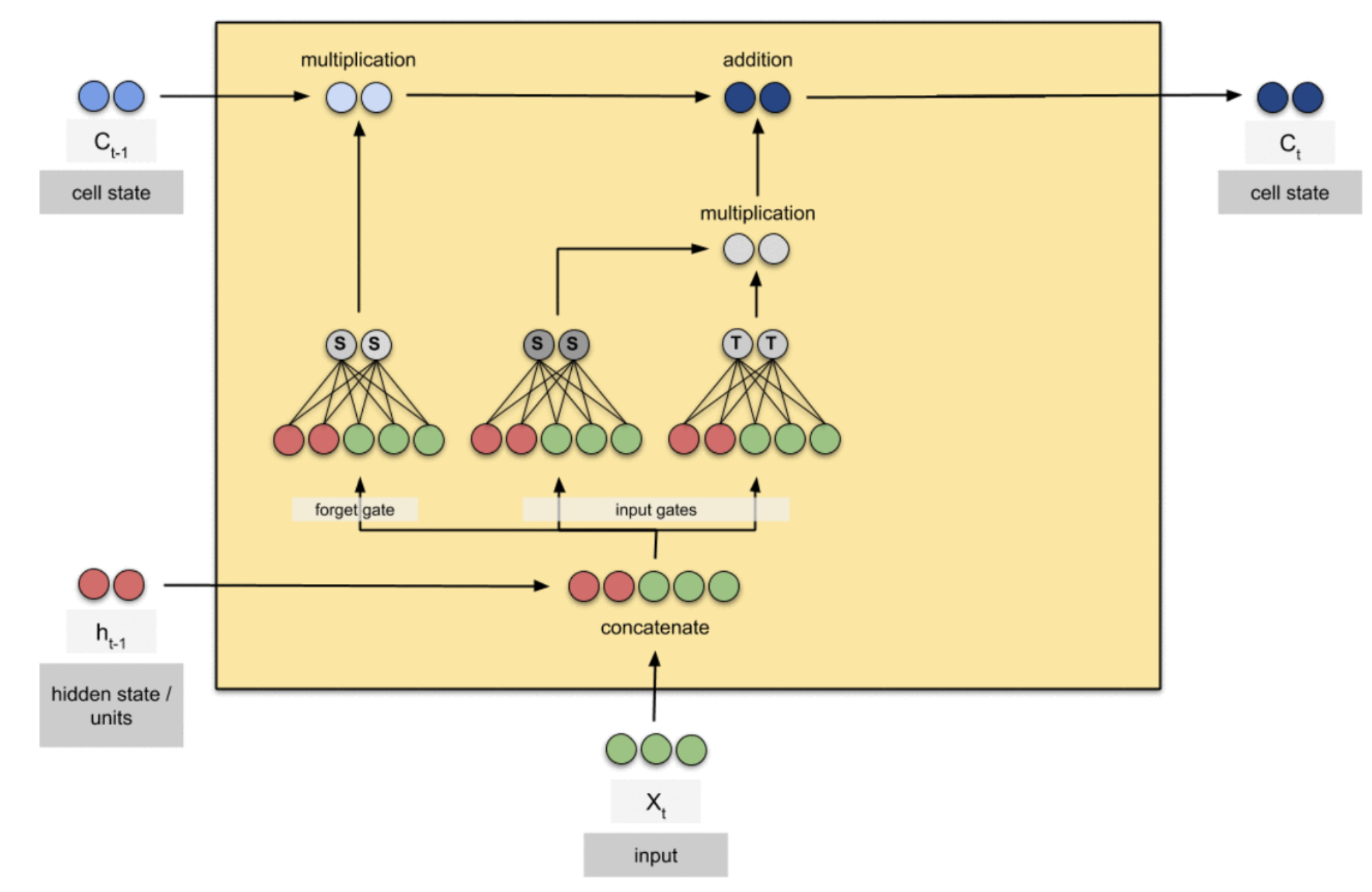
Cell state update combines retained past memory (via the forget gate) with selected new information (via the input gate and candidate state) to produce the updated long-term memory.
\[ c_1 = f_1 \odot c_0 + i_1 \odot \tilde{c}_1 \]
We have our historic information \[ h_0 = \begin{bmatrix}0\\0\end{bmatrix}, \quad c_0 = \begin{bmatrix}0\\0\end{bmatrix} \]
 \[
c_1 = f_1 \odot c_0 + i_1 \odot \tilde{c}_1
\]
Since \(c_0 = [0,0]^T\): \[ c_1 = \begin{bmatrix}0\\0\end{bmatrix} + \begin{bmatrix}0.881\\0.500\end{bmatrix} \odot \begin{bmatrix}0.762\\0.762\end{bmatrix} \]
\[ c_1 \approx\left[\begin{array}{l} 0.671 \\ 0.381 \end{array}\right] \]
Output gate
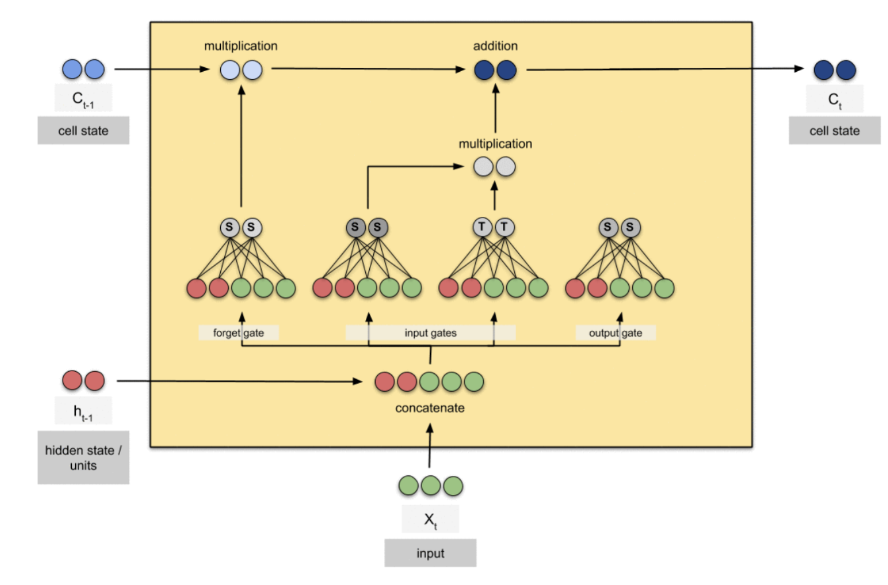
Output gate decides how much of the current cell state should be exposed as the hidden state/output.
\[ o_t=\sigma\left(W_o x_t+U_o h_{t-1}+b_o\right) \\ \]
\[ W_o = \begin{bmatrix} 1 & 0 & 1 \\ 1 & 1 & 0 \end{bmatrix}, \qquad U_o = \begin{bmatrix} 1 & 1 \\ 0 & 1 \end{bmatrix}, \qquad b_o = \begin{bmatrix} 0\\1 \end{bmatrix} \]
\[ W_o x_1 = \begin{bmatrix} 1 & 0 & 1 \\ 1 & 1 & 0 \end{bmatrix} \begin{bmatrix}1\\0\\0\end{bmatrix} = \begin{bmatrix}1\\1\end{bmatrix} \]
So: \[ W_o x_1 + U_o h_0 + b_o = \begin{bmatrix}1\\1\end{bmatrix} + \begin{bmatrix}0\\0\end{bmatrix} + \begin{bmatrix}0\\1\end{bmatrix} = \begin{bmatrix}1\\2\end{bmatrix} \] Thus: \[ o_1 = \sigma\left(\begin{bmatrix}1\\2\end{bmatrix}\right) = \begin{bmatrix}0.731\\0.881\end{bmatrix} \]
Word-2: eat
… and the process repeats itself with out updated history terms (i.e. recurrence)
Step 2: process eat
\[ x_2 = \begin{bmatrix}0\\1\\0\end{bmatrix} \]
Forget gate
\[ W_f x_2 = \begin{bmatrix} 1 & 0 & 0 \\ 0 & 1 & 1 \end{bmatrix} \begin{bmatrix}0\\1\\0\end{bmatrix} = \begin{bmatrix}0\\1\end{bmatrix} \]
So pre-activation: \[ \begin{bmatrix}0\\1\end{bmatrix} + \begin{bmatrix}0.428\\0.321\end{bmatrix} + \begin{bmatrix}0\\1\end{bmatrix} = \begin{bmatrix}0.428\\2.321\end{bmatrix} \] Therefore: \[ f_2 \approx \begin{bmatrix} \sigma(0.428)\\ \sigma(2.321) \end{bmatrix} \approx \begin{bmatrix} 0.605\\ 0.911 \end{bmatrix} \]
Input gate
\[ W_i x_2 = \begin{bmatrix} 1 & 1 & 0 \\ 0 & 1 & 1 \end{bmatrix} \begin{bmatrix}0\\1\\0\end{bmatrix} = \begin{bmatrix}1\\1\end{bmatrix} \]
So pre-activation: \[ \begin{bmatrix}1\\1\end{bmatrix} + \begin{bmatrix}0.428\\0.749\end{bmatrix} + \begin{bmatrix}1\\0\end{bmatrix} = \begin{bmatrix}2.428\\1.749\end{bmatrix} \] Hence: \[ i_2 \approx \begin{bmatrix} 0.919\\ 0.852 \end{bmatrix} \]
Candidate cell state
\[ W_c x_2 = \begin{bmatrix} 1 & 0 & 1 \\ 0 & 1 & 1 \end{bmatrix} \begin{bmatrix}0\\1\\0\end{bmatrix} = \begin{bmatrix}0\\1\end{bmatrix} \]
So pre-activation: \[ \begin{bmatrix}0\\1\end{bmatrix} + \begin{bmatrix}0.428\\0.321\end{bmatrix} + \begin{bmatrix}0\\1\end{bmatrix} = \begin{bmatrix}0.428\\2.321\end{bmatrix} \] Thus: \[ \tilde{c}_2 \approx \begin{bmatrix} \tanh(0.428)\\ \tanh(2.321) \end{bmatrix} \approx \begin{bmatrix} 0.404\\ 0.981 \end{bmatrix} \]
Cell update
\[ c_2 = f_2 \odot c_1 + i_2 \odot \tilde{c}_2 \]
First term: \[ f_2 \odot c_1 \approx \begin{bmatrix} 0.605\\ 0.911 \end{bmatrix} \odot \begin{bmatrix} 0.671\\ 0.381 \end{bmatrix} = \begin{bmatrix} 0.406\\ 0.347 \end{bmatrix} \] Second term: \[ i_2 \odot \tilde{c}_2 \approx \begin{bmatrix} 0.919\\ 0.852 \end{bmatrix} \odot \begin{bmatrix} 0.404\\ 0.981 \end{bmatrix} = \begin{bmatrix} 0.371\\ 0.836 \end{bmatrix} \] So: \[ c_2 \approx \begin{bmatrix} 0.777\\ 1.183 \end{bmatrix} \]
Output gate
\[ W_o x_2 = \begin{bmatrix} 1 & 0 & 1 \\ 1 & 1 & 0 \end{bmatrix} \begin{bmatrix}0\\1\\0\end{bmatrix} = \begin{bmatrix}0\\1\end{bmatrix} \]
So pre-activation: \[ \begin{bmatrix}0\\1\end{bmatrix} + \begin{bmatrix}0.749\\0.321\end{bmatrix} + \begin{bmatrix}0\\1\end{bmatrix} = \begin{bmatrix}0.749\\2.321\end{bmatrix} \] Thus: \[ o_2 \approx \begin{bmatrix} 0.679\\ 0.911 \end{bmatrix} \]
Word-3: Bread
Step 3: process bread
\[ x_3 = \begin{bmatrix}0\\0\\1\end{bmatrix} \]
Forget gate
\[ W_f x_3 = \begin{bmatrix} 1 & 0 & 0 \\ 0 & 1 & 1 \end{bmatrix} \begin{bmatrix}0\\0\\1\end{bmatrix} = \begin{bmatrix}0\\1\end{bmatrix} \]
So pre-activation: \[ \begin{bmatrix}0\\1\end{bmatrix} + \begin{bmatrix}0.442\\0.754\end{bmatrix} + \begin{bmatrix}0\\1\end{bmatrix} = \begin{bmatrix}0.442\\2.754\end{bmatrix} \] Hence: \[ f_3 \approx \begin{bmatrix} 0.609\\ 0.940 \end{bmatrix} \]
Input gate
\[ W_i x_3 = \begin{bmatrix} 1 & 1 & 0 \\ 0 & 1 & 1 \end{bmatrix} \begin{bmatrix}0\\0\\1\end{bmatrix} = \begin{bmatrix}0\\1\end{bmatrix} \]
So pre-activation: \[ \begin{bmatrix}0\\1\end{bmatrix} + \begin{bmatrix}0.442\\1.196\end{bmatrix} + \begin{bmatrix}1\\0\end{bmatrix} = \begin{bmatrix}1.442\\2.196\end{bmatrix} \] Thus: \[ i_3 \approx \begin{bmatrix} 0.809\\ 0.900 \end{bmatrix} \]
Candidate cell state
\[ W_c x_3 = \begin{bmatrix} 1 & 0 & 1 \\ 0 & 1 & 1 \end{bmatrix} \begin{bmatrix}0\\0\\1\end{bmatrix} = \begin{bmatrix}1\\1\end{bmatrix} \]
So pre-activation: \[ \begin{bmatrix}1\\1\end{bmatrix} + \begin{bmatrix}0.442\\0.754\end{bmatrix} + \begin{bmatrix}0\\1\end{bmatrix} = \begin{bmatrix}1.442\\2.754\end{bmatrix} \] Thus: \[ \tilde{c}_3 \approx \begin{bmatrix} 0.894\\ 0.992 \end{bmatrix} \]
Cell update
\[ c_3 = f_3 \odot c_2 + i_3 \odot \tilde{c}_3 \]
First term: \[ f_3 \odot c_2 \approx \begin{bmatrix} 0.609\\ 0.940 \end{bmatrix} \odot \begin{bmatrix} 0.777\\ 1.183 \end{bmatrix} = \begin{bmatrix} 0.473\\ 1.112 \end{bmatrix} \] Second term: \[ i_3 \odot \tilde{c}_3 \approx \begin{bmatrix} 0.809\\ 0.900 \end{bmatrix} \odot \begin{bmatrix} 0.894\\ 0.992 \end{bmatrix} = \begin{bmatrix} 0.723\\ 0.893 \end{bmatrix} \] So: \[ c_3 \approx \begin{bmatrix} 1.196\\ 2.005 \end{bmatrix} \]
Output gate
\[ W_o x_3 = \begin{bmatrix} 1 & 0 & 1 \\ 1 & 1 & 0 \end{bmatrix} \begin{bmatrix}0\\0\\1\end{bmatrix} = \begin{bmatrix}1\\0\end{bmatrix} \]
So pre-activation: \[ \begin{bmatrix}1\\0\end{bmatrix} + \begin{bmatrix}1.196\\0.754\end{bmatrix} + \begin{bmatrix}0\\1\end{bmatrix} = \begin{bmatrix}2.196\\1.754\end{bmatrix} \] Thus: \[ o_3 \approx \begin{bmatrix} 0.900\\ 0.852 \end{bmatrix} \]
LSTM Architecture
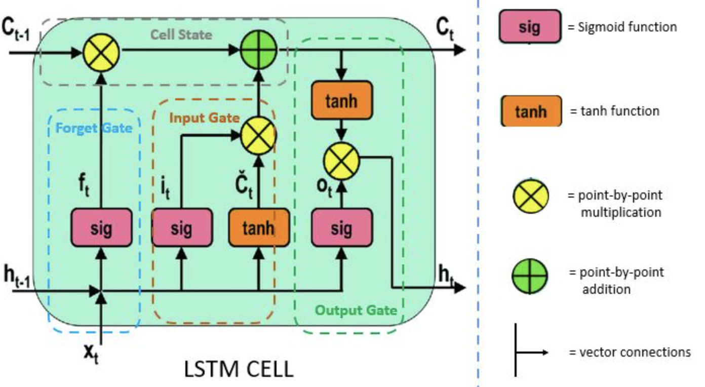
Overview
Designed to learn long-range dependencies in sequences by addressing vanishing/exploding gradients seen in vanilla RNNs.
Key Components and computations
Core Components (per time step \(t\) )
- Cell state \(C_t\) : long-term memory that flows through the network.
- Hidden state \(h_t\) : short-term representation used for outputs.
- Gates (sigmoid activations) control information flow:
- Forget gate \(f_t\) : decides what information to discard.
- Input gate \(i_t\) : decides what new information to store.
- Output gate \(o_t\) : controls what part of the cell state becomes output.
Key Computations
- Forget: \(f_t=\sigma\left(W_f\left[h_{t-1}, x_t\right]+b_f\right)\)
- Input: \(i_t=\sigma\left(W_i\left[h_{t-1}, x_t\right]+b_i\right)\)
- Candidate memory: \(\tilde{C}_t=\tanh \left(W_c\left[h_{t-1}, x_t\right]+b_c\right)\)
- Cell update: \(C_t=f_t \odot C_{t-1}+i_t \odot \tilde{C}_t\)
- Output: \(h_t=o_t \odot \tanh \left(C_t\right)\)
tanh squashes values to [-1, 1], keeping activations stable and bounded as information moves in or out of the cell state.
I know that is alot, let’s break it down.
Cell state
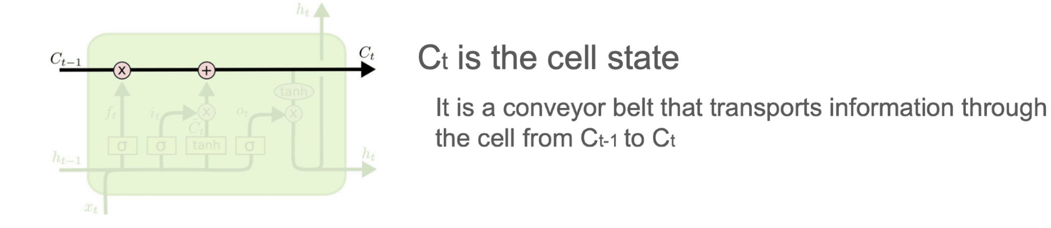
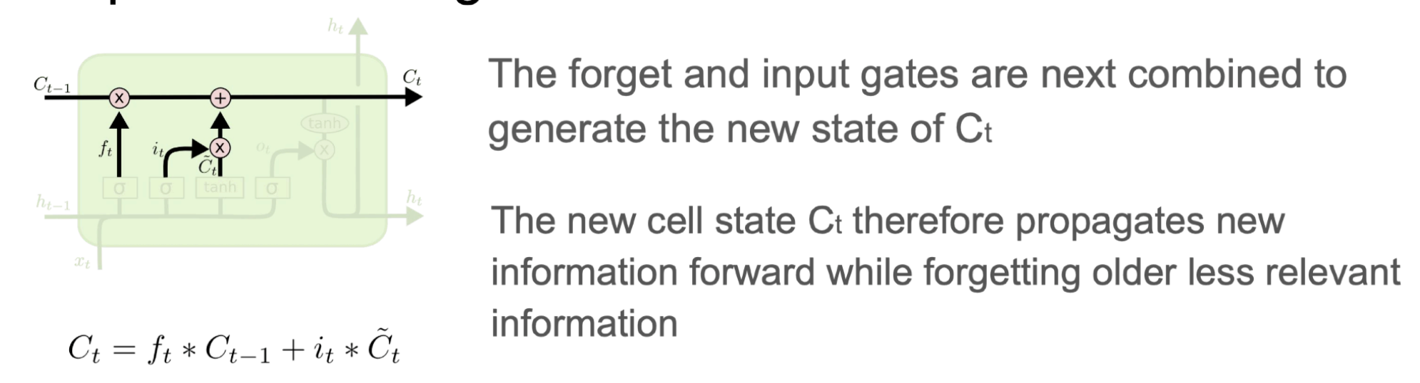
- The cell state acts as the LSTM’s long-term memory, carrying information across time steps.
- Information flows with little modification, enabling long-range dependencies.
- Additive updates help preserve gradient flow. Information can be added or removed via the additive cell update.
- Cell update: \(C_t=f_t \odot C_{t-1}+i_t \odot \tilde{C}_t\)
- The forget gate discards unneeded prior information.
- The input gate determines which new information to store.
- Serves as the main
information highwaythrough the sequence. - The output gate controls how much of the cell state affects the hidden state \(h_t\).
Purpose of gated units
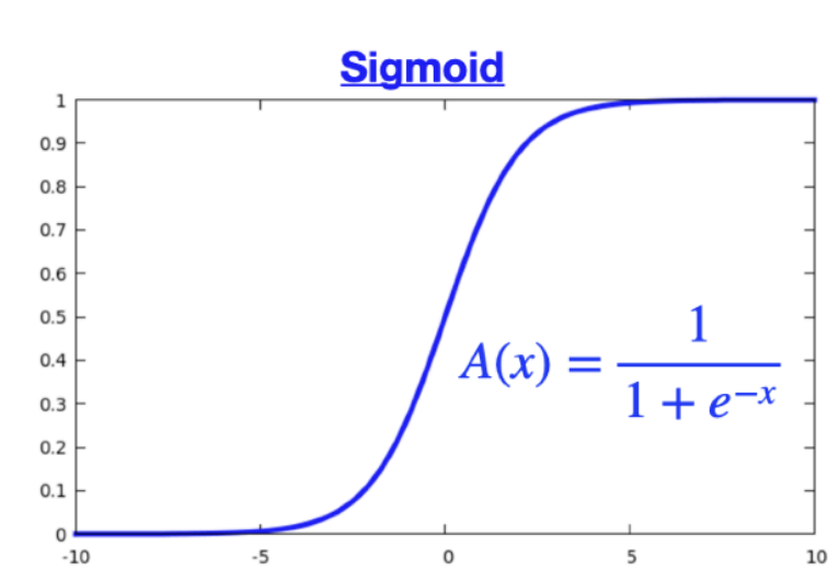
Gates regulate memory, allowing gradients & information to transverse many time steps.
Gates regulate memory, allowing gradients and information to flow across many time steps.
Gates scale signals multiplicatively (attenuation).
Each gate outputs a value in [0,1], controlling how much information passes.
Therefore gates use the sigmoid activation function.
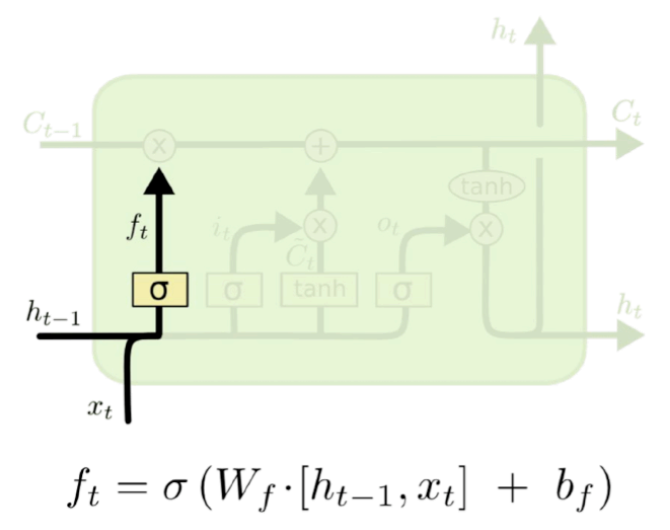
Evaluation: Step 1 - Forget Gate
Goal: decide how much information from the previous cell state should be retained.
- The forget gate determines how much information from the previous cell state should be retained.
- It outputs values between \(\mathbf{0}\) and 1, acting as a soft filter on past memory.
- \(\mathbf{0} \boldsymbol{\rightarrow}\) forget the information, \(\mathbf{1} \boldsymbol{\rightarrow}\) fully keep it.
- This down-weights irrelevant or outdated information while preserving useful context.
- The gate scales the previous cell state before the update.
Cell update:
\[ C_t=f_t \odot C_{t-1}+i_t \odot \tilde{C}_t \]
Evaluation: Step 2- Input Gate
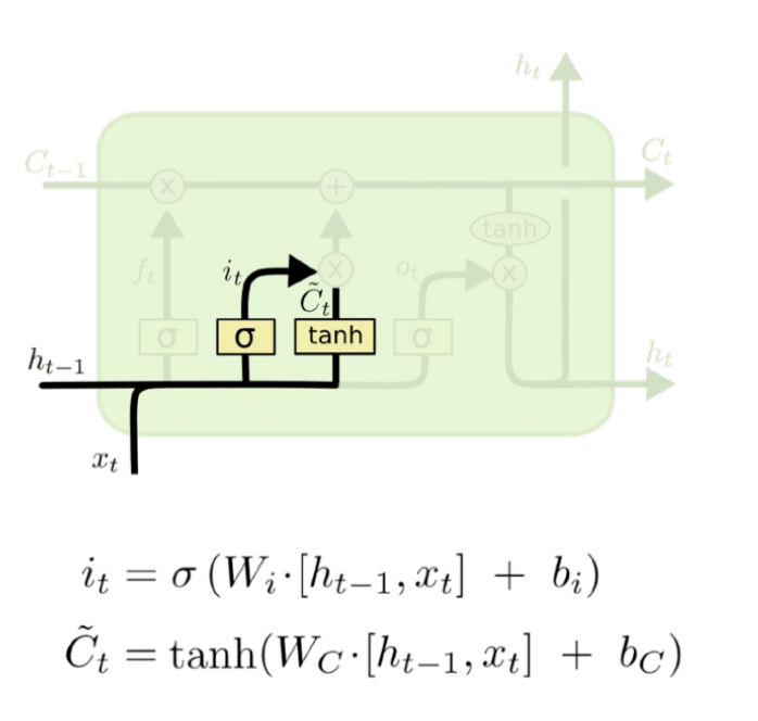
Goal: decide what new information to store
- The input gate determines what new information will be added to the cell state.
- A sigmoid layer decides which components should be updated.
- A tanh layer generates a candidate vector of new values.
- The gate output and candidate values are combined to form the update to the cell state.
Candidate Cell State \(\tilde{C}_t\)
- The candidate represents new information the network proposes to store in the cell state.
- It is computed from the current input \(x_t\) and previous hidden state \(h_{t-1}\).
- A tanh activation produces values in \([-1,1]\), allowing both positive and negative updates to memory.
- This vector contains potential content, but it is not written directly to the cell state.
- Instead, the input gate \(i_t\) scales it, determining how much of the candidate is actually stored.
\[ \tilde{C}_t=\tanh \left(W_c\left[h_{t-1}, x_t\right]+b_c\right) \]
Evaluation: Step 3 Combining information
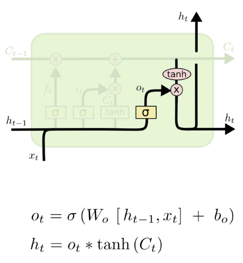
Evaluation: Step 4: Value resolution and information passing
Once the cell state is updated 3 things occur:
- Ct is multiplied by a sigmoid “output gate” (sigmoid) which decides on the relevant information to output
- The outpute gate is then scaled by a tanh function
- Finally the new hidden state is output and also passed along to \(\mathrm{C}_{\mathrm{t}+1}\)
LSTM GIF Animation
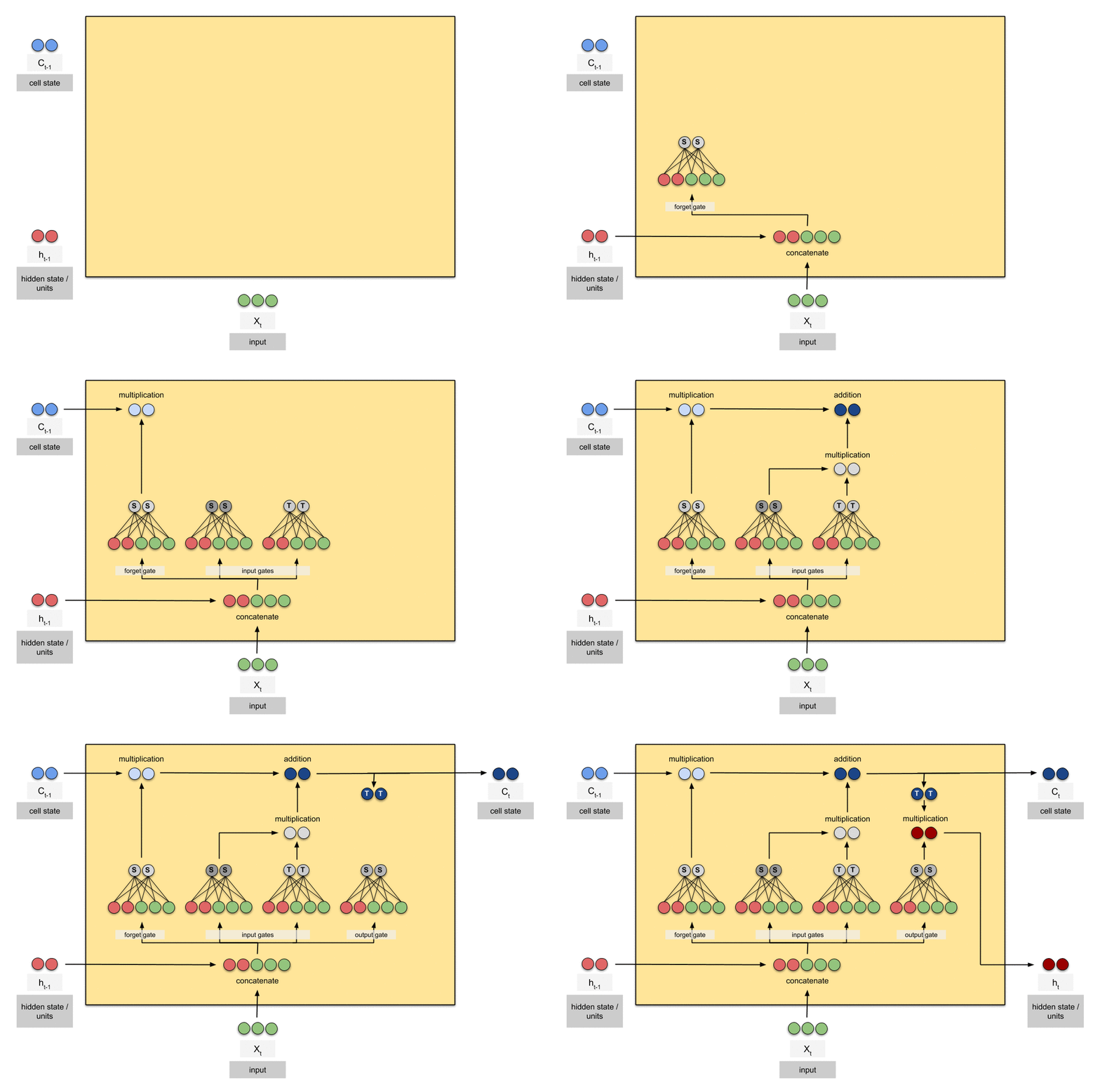
Source: https://medium.com/data-science/animated-rnn-lstm-and-gru-ef124d06cf45
Summary
images/2026-03-11-12-25-23.png
GRU: Gated Recurrent Units
Overview
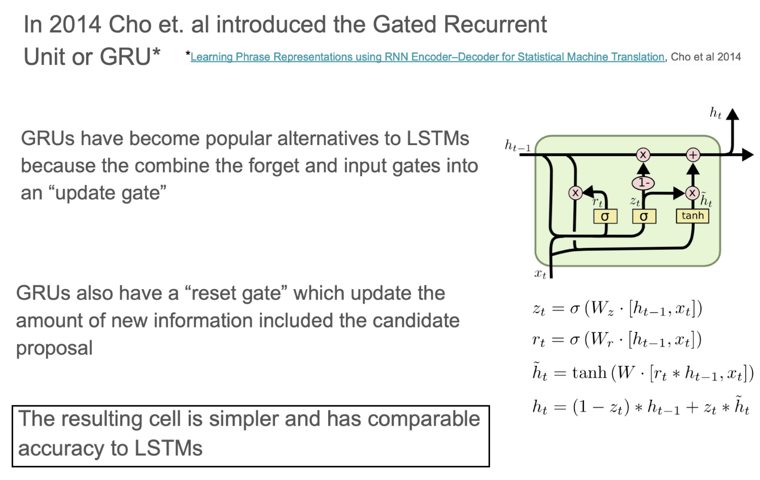
GRU GIF Animation
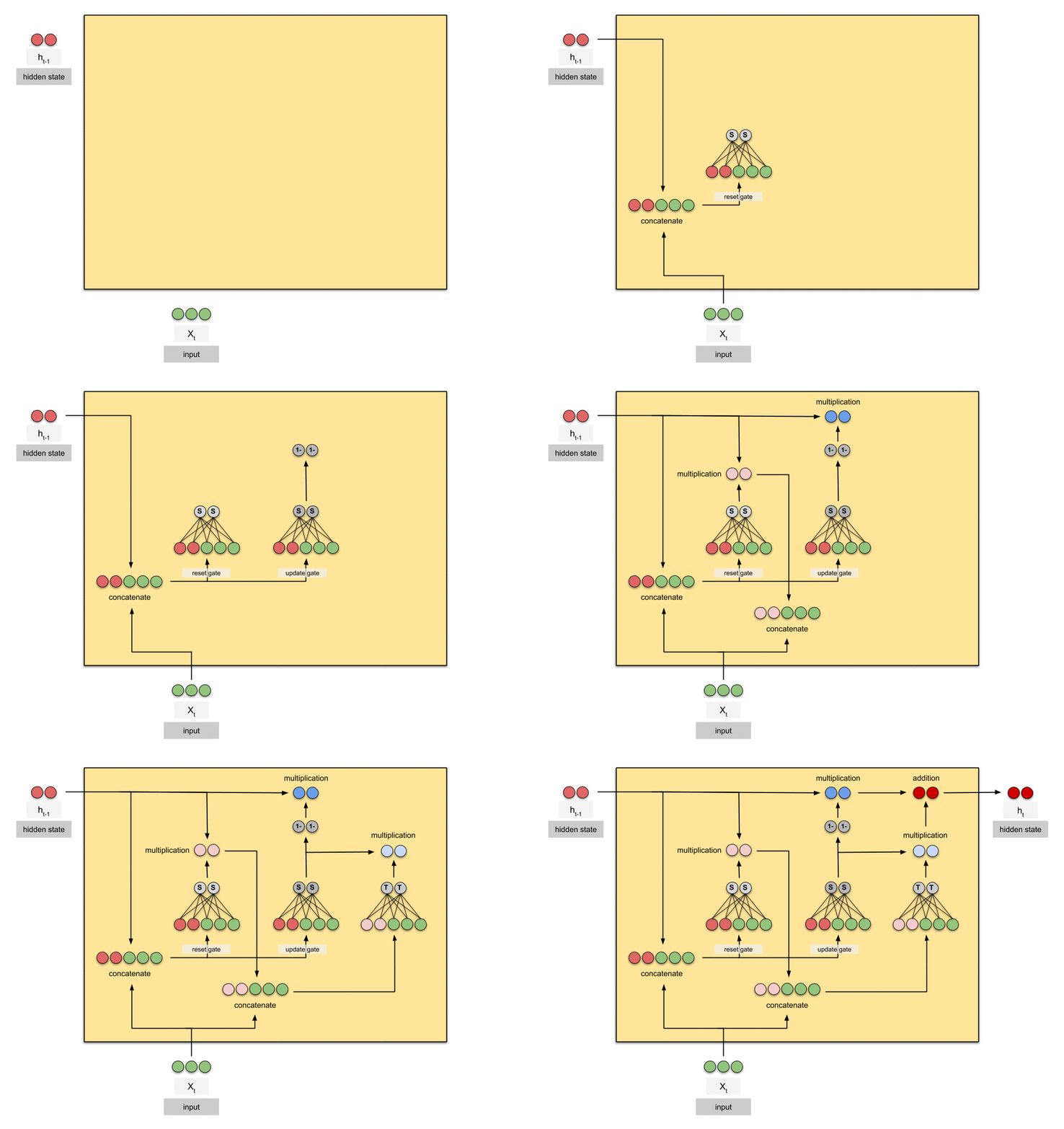
Source: https://medium.com/data-science/animated-rnn-lstm-and-gru-ef124d06cf45
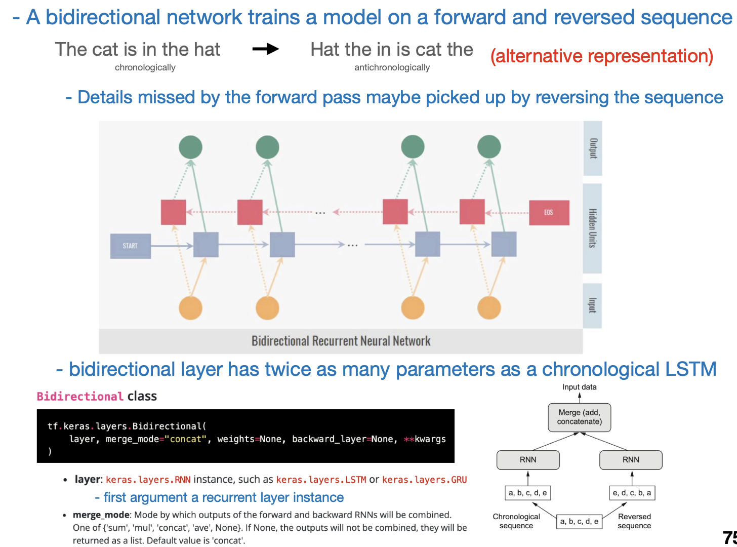
Aside: Bi-directional RNNs