Both libraries are built on a single idea: the n-dimensional array — a grid of numbers, all of the same type, stored in one contiguous block of memory.
Working with a grid as a whole object (instead of looping over it) is what makes scientific Python fast and readable. Learn the idea once in NumPy, and PyTorch is mostly the same idea with two superpowers added: it can run on a GPU, and it can compute derivatives automatically.
Section 1: NumPy Arrays
1.1 Why not just use Python lists?
A Python list is a flexible bag of pointers to arbitrary objects. A NumPy array is a rigid block of raw numbers. Rigidity buys speed and gives us vectorized operations: one line acts on every element.
import numpy as npnums = [1, 2, 3, 4]# A list "multiplied" repeats itself, and elementwise math needs a loop.print("list * 2 :", nums *2)print("loop doubling :", [x *2for x in nums])# An array behaves like a mathematical vector.arr = np.array(nums)print("array * 2 :", arr *2)print("array + array :", arr + arr)
# The speed difference is the reason we care.big_list =list(range(1_000_000))big_arr = np.arange(1_000_000)%timeit sum(x * x for x in big_list)%timeit (big_arr **2).sum()
34.3 ms ± 1.18 ms per loop (mean ± std. dev. of 7 runs, 10 loops each)
1.08 ms ± 28.8 μs per loop (mean ± std. dev. of 7 runs, 1,000 loops each)
1.2 Creating arrays
Beyond np.array(...), most arrays come from a handful of factory functions.
rng = np.random.default_rng(seed=0) # reproducible randomnessprint(np.zeros(3)) # [0. 0. 0.]print(np.ones((2, 3))) # 2 rows, 3 columns of 1.0print(np.arange(0, 10, 2)) # like range(): start, stop, stepprint(np.linspace(0, 1, 5)) # 5 evenly spaced points, endpoints includedprint(np.eye(3)) # identity matrixprint(rng.normal(size=(2, 2))) # samples from a standard normal
Every array carries its own description. shape is the one you will check a hundred times a day.
X = np.array([[1.0, 2.0, 3.0], [4.0, 5.0, 6.0]])print("shape:", X.shape) # (rows, columns)print("ndim :", X.ndim) # number of axes/dimensionsprint("size :", X.size) # total number of elementsprint("dtype:", X.dtype) # the single type shared by all elements
shape: (2, 3)
ndim : 2
size : 6
dtype: float64
The dtype is fixed at creation. If you build an array from integers, it stores integers — and assignments get silently truncated to fit.
ints = np.array([1, 2, 3])print(ints.dtype)ints[0] =3.99# truncated, not rounded, to fit an int arrayprint(ints)floats = ints.astype(np.float64) # .astype() makes a converted copyfloats[0] =3.99print(floats, floats.dtype)
int64
[3 2 3]
[3.99 2.   3.  ] float64
1.4 Indexing and slicing
Index with one number per axis: X[row, col]. A slice start:stop takes everything up to but not includingstop. A bare : means “the whole axis.”
X = np.arange(12).reshape(3, 4)print(X)print("\nX[1, 2] ->", X[1, 2]) # single element: row 1, column 2print("X[0] ->", X[0]) # entire first rowprint("X[:, 1] ->", X[:, 1]) # entire second columnprint("X[0:2, 1:3] ->\n", X[0:2, 1:3]) # a 2x2 sub-block
A slice is a view, not a copy. It looks into the original array’s memory. Writing to it writes to the original. This is a feature (no wasted memory) and a classic source of bugs.
a = np.arange(6)view = a[1:4]view[0] =99print("a after writing to a view:", a)b = np.arange(6)copy = b[1:4].copy() # ask explicitly for independent memorycopy[0] =99print("b after writing to a copy:", b)
a after writing to a view: [ 0 99  2  3  4  5]
b after writing to a copy: [0 1 2 3 4 5]
1.5 Broadcasting
Operations happen elementwise. When shapes differ, NumPy stretches the smaller one — without ever copying the data — as long as each axis is either equal in size or of length 1.
A (3, 1) column plus a (1, 4) row both stretch to (3, 4):
# The everyday case: a scalar or a single row applied to a whole matrix.X = np.array([[1.0, 2.0, 3.0], [4.0, 5.0, 6.0]])print(X *10) # scalar broadcasts to every elementprint(X - np.array([1.0, 1.0, 0.0])) # one row broadcasts down all rows
reshape reinterprets the same numbers under a new shape; the element count must match. Use -1 for “you figure this dimension out.”
v = np.arange(6)print(v.reshape(2, 3))print(v.reshape(3, -1)) # -1 is inferred as 2M = np.arange(6).reshape(2, 3)print("\nM.T has shape", M.T.shape)print(M.T)
* is elementwise. @ is the linear-algebra matrix product. Confusing them is the single most common NumPy error.
A = np.array([[1, 2], [3, 4]])B = np.array([[10, 0], [0, 10]])print("A * B (elementwise):\n", A * B)print("\nA @ B (matrix product):\n", A @ B)# Shapes must line up: (2,3) @ (3,) -> (2,)M = np.arange(6).reshape(2, 3)x = np.array([1, 0, -1])print("\nM @ x ->", M @ x)
A * B (elementwise):
 [[10  0]
 [ 0 40]]

A @ B (matrix product):
 [[10 20]
 [30 40]]

M @ x -> [-2 -2]
1.9 Boolean masks
Comparisons produce arrays of True/False, which can then be used to select or overwrite elements. This replaces most if statements inside loops.
data = np.array([3.0, -1.0, 4.0, -1.5, 0.0, 2.5])mask = data >0print("mask :", mask)print("data[mask] :", data[mask]) # keep only the elements where mask is Trueprint("count > 0 :", mask.sum()) # True counts as 1print("any / all :", mask.any(), mask.all())clipped = data.copy()clipped[clipped <0] =0# ReLU, in one lineprint("clipped :", clipped)
A typical preprocessing step. Rows are samples, columns are features; we rescale each feature to have mean 0 and standard deviation 1. Broadcasting and axis do all the work.
rng = np.random.default_rng(0)data = rng.normal(loc=[100.0, 0.5], scale=[15.0, 0.1], size=(1000, 2))mu = data.mean(axis=0) # shape (2,) — one mean per featuresigma = data.std(axis=0) # shape (2,) — one std per featurestandardized = (data - mu) / sigma # (1000, 2) - (2,) broadcasts down every rowprint("original mean/std :", mu.round(3), sigma.round(3))print("new mean/std :", standardized.mean(axis=0).round(3), standardized.std(axis=0).round(3))
original mean/std : [99.551  0.497] [15.289  0.098]
new mean/std      : [-0. -0.] [1. 1.]
Section 2: PyTorch Tensors
A torch.Tensor is the same object as a NumPy array — a typed n-dimensional grid — with the same creation functions, the same indexing, the same broadcasting, the same axis reductions (spelled dim), and the same @.
What it adds:
It can live on a GPU.
It can track the operations performed on it and compute derivatives with respect to it, automatically. This is what makes neural networks trainable.
2.1 The familiar half
If you know Section 1, you already know this section. Almost everything transfers.
A tensor lives on a device. Moving it to a GPU makes the same operations run in parallel over thousands of cores. The standard, portable idiom:
device ="cuda"if torch.cuda.is_available() else"cpu"print("using device:", device)x = torch.randn(3, 3).to(device)y = torch.randn(3, 3).to(device)z = x @ y # runs on the GPU if one is availableprint(z.device)# Note: tensors must be on the SAME device to interact.
using device: cpu
cpu
2.4 Autograd: the real reason PyTorch exists
Set requires_grad=True and the tensor starts recording every operation it takes part in, building a graph. Calling .backward() on a scalar result walks that graph backwards and deposits \(\partial(\text{result}) / \partial(\text{each input})\) into each input’s .grad.
Take \(y = x^2 + 3x\). Calculus says \(dy/dx = 2x + 3\), so at \(x = 2\) the derivative is \(7\). PyTorch should agree.
x = torch.tensor(2.0, requires_grad=True)y = x**2+3*x # forward pass: torch quietly records what happenedy.backward() # backward pass: differentiate y with respect to xprint("y =", y.item())print("dy/dx =", x.grad.item(), " (analytic answer: 2*2 + 3 = 7)")
This works for any number of inputs at once, which is the whole trick: a neural network is just a function of millions of parameters, and .backward() gets the derivative with respect to every one of them in a single pass.
w = torch.tensor([1.0, 2.0], requires_grad=True)b = torch.tensor(0.5, requires_grad=True)x = torch.tensor([3.0, 4.0])loss = ((w @ x + b) -10.0)**2# a scalarloss.backward()print("dloss/dw =", w.grad) # one gradient per parameterprint("dloss/db =", b.grad)
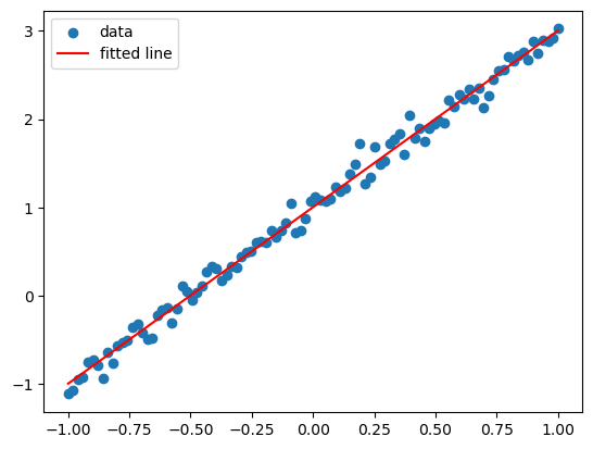
Everything above, combined: fit a line \(y = wx + b\) to noisy data generated from \(y = 2x + 1\). The loop is gradient descent — nudge each parameter in the direction that decreases the loss.
Three things to notice:
loss.backward() fills in .grad for w and b.
Updates happen under torch.no_grad() because adjusting the parameters is bookkeeping, not part of the function we are differentiating.
Gradients accumulate by default, so we zero them each step.
torch.manual_seed(0)x = torch.linspace(-1, 1, 100)y =2*x +1+0.1*torch.randn(100) # true parameters: w = 2, b = 1w = torch.tensor(0.0, requires_grad=True)b = torch.tensor(0.0, requires_grad=True)lr =0.1for step inrange(101): y_pred = w * x + b # forward loss = ((y_pred - y)**2).mean() # mean squared error loss.backward() # compute dloss/dw and dloss/dbwith torch.no_grad(): # update, untracked w -= lr * w.grad b -= lr * b.grad w.grad.zero_() # reset for the next step b.grad.zero_()if step %25==0:print(f"step {step:3d} | loss {loss.item():.4f} | w {w.item():.3f} | b {b.item():.3f}")print("\nrecovered w, b =", round(w.item(), 3), round(b.item(), 3), " (truth: 2.0, 1.0)")
step   0 | loss 2.3780 | w 0.136 | b 0.201
step  25 | loss 0.0507 | w 1.679 | b 1.001
step  50 | loss 0.0117 | w 1.945 | b 1.004
step  75 | loss 0.0105 | w 1.990 | b 1.004
step 100 | loss 0.0105 | w 1.998 | b 1.004

recovered w, b = 1.998 1.004  (truth: 2.0, 1.0)