Pick a device — GPU if available, otherwise CPU. Tensors and models must live on the same device.
Set a random seed so results are reproducible (weights are initialized randomly!).
import torchimport torch.nn as nnimport torch.optim as optimfrom torch.utils.data import DataLoader, random_splitimport torchvisionimport torchvision.transforms as transformsimport numpy as npimport matplotlib.pyplot as plttorch.manual_seed(42) # reproducibilitynp.random.seed(42)device ="cuda"if torch.cuda.is_available() else"cpu"print("PyTorch version:", torch.__version__)print("Using device:", device)
PyTorch version: 2.8.0
Using device: cpu
Step 1 — Load the data
A PyTorch Dataset is just an object that answers two questions: - How many samples do you have? (len(dataset)) - Give me sample i. (dataset[i] → (image, label))
MNIST ships with torchvision, so we get it for free. The transform converts each PIL image into a tensor and normalizes it:
ToTensor() → shape (1, 28, 28), pixel values scaled from 0-255 to 0.0-1.0.
Normalize(mean, std) → recenters pixels to roughly mean 0, std 1. Networks train faster and more stably when inputs are on a standard scale. (0.1307 and 0.3081 are the well-known MNIST statistics.)
transform = transforms.Compose([ transforms.ToTensor(), # PIL image -> tensor in [0, 1] transforms.Normalize((0.1307,), (0.3081,)) # standardize: (x - mean) / std])# MNIST comes pre-split into an official train set and test set.full_train = torchvision.datasets.MNIST(root="./data", train=True, download=True, transform=transform)test_set = torchvision.datasets.MNIST(root="./data", train=False, download=True, transform=transform)print("Training images (before val split):", len(full_train))print("Test images:", len(test_set))
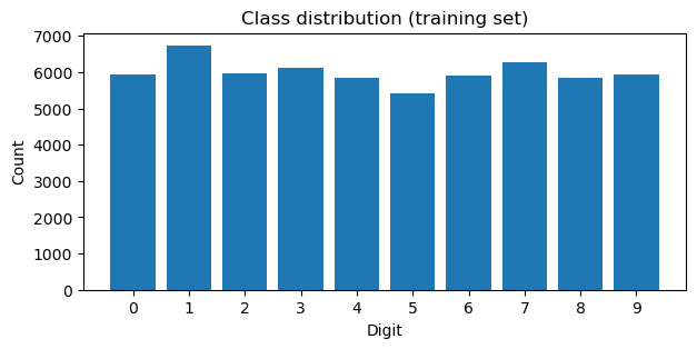
# Class balance: how many of each digit?labels = full_train.targets.numpy()counts = np.bincount(labels)plt.figure(figsize=(7, 3))plt.bar(range(10), counts)plt.xticks(range(10))plt.xlabel("Digit"); plt.ylabel("Count"); plt.title("Class distribution (training set)")plt.show()print("Min class count:", counts.min(), "| Max class count:", counts.max())
Min class count: 5421 | Max class count: 6742
Takeaway: the classes are roughly balanced (~6,000 each), so plain accuracy is a fair metric here. If one class were 90% of the data, accuracy would be misleading and we would need precision/recall instead.
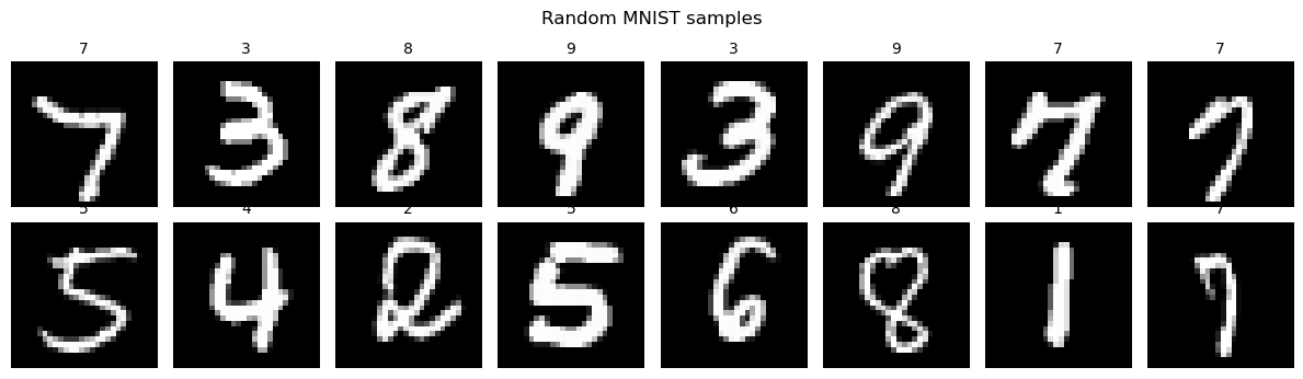
Visualize some digits
Undo the normalization before plotting, otherwise the image looks washed out.
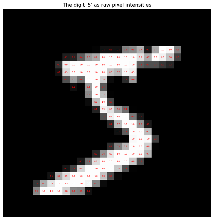
# A digit is just a 28x28 grid of numbers. Here is what the model actually "sees".img, lab = full_train[0]pixels = unnormalize(img).squeeze().numpy()fig, ax = plt.subplots(figsize=(9, 9))ax.imshow(pixels, cmap="gray")for i inrange(28):for j inrange(28): v = pixels[i, j]if v >0.05: # skip the empty background for readability ax.text(j, i, f"{v:.1f}", ha="center", va="center", fontsize=5, color="red")ax.set_title(f"The digit '{lab}' as raw pixel intensities")ax.axis("off")plt.show()
Step 3 — Split into training and validation
We have three roles for data:
Train (~85%) — the model updates its weights on this.
Validation (~15%) — held out from training; used to watch for overfitting and make decisions (when to stop, which architecture).
Test — touched once, at the very end, to report an honest final number.
A Dataset gives you one sample at a time. A DataLoader wraps it and handles the boring-but-essential mechanics:
Batching — stacks 64 samples into one tensor of shape (64, 1, 28, 28). GPUs are fast because they process a batch in parallel.
Shuffling — reshuffles the training data every epoch so the model does not memorize the sample order. (No need to shuffle val/test — we are only reading from them.)
Iteration — you just write for X, y in train_loader:.
BATCH_SIZE =64train_loader = DataLoader(train_set, batch_size=BATCH_SIZE, shuffle=True)val_loader = DataLoader(val_set, batch_size=BATCH_SIZE, shuffle=False)test_loader = DataLoader(test_set, batch_size=BATCH_SIZE, shuffle=False)# Peek at exactly what one iteration hands us:X_batch, y_batch =next(iter(train_loader))print("X_batch shape:", X_batch.shape, " <- (batch, channels, height, width)")print("y_batch shape:", y_batch.shape, " <- one integer label per image")print("Batches per epoch:", len(train_loader))
X_batch shape: torch.Size([64, 1, 28, 28])  <- (batch, channels, height, width)
y_batch shape: torch.Size([64])  <- one integer label per image
Batches per epoch: 797
Step 5 — Define the model
A multi-layer perceptron (MLP) is a stack of fully-connected layers with a nonlinearity in between.
# Sanity check BEFORE training: does one batch flow through and come out the right shape?with torch.no_grad(): logits = model(X_batch.to(device))print("Input :", X_batch.shape)print("Output:", logits.shape, " <- 10 scores per image")print("\nLogits for the first image:\n", logits[0].cpu().numpy().round(2))print("Predicted class (argmax):", logits[0].argmax().item(), "| True:", y_batch[0].item())print("\n(Untrained -> essentially a random guess. That's expected.)")
Input : torch.Size([64, 1, 28, 28])
Output: torch.Size([64, 10])  <- 10 scores per image

Logits for the first image:
 [ 0.06  0.05  0.    0.11 -0.06  0.11 -0.05 -0.06  0.03  0.01]
Predicted class (argmax): 3 | True: 8

(Untrained -> essentially a random guess. That's expected.)
Step 6 — Loss function and optimizer
Loss = how wrong we are. CrossEntropyLoss is the standard for multi-class classification: it softmaxes the logits into probabilities and penalizes low probability on the true class.
Optimizer = how we fix it. It reads the gradients and nudges each weight downhill. Adam is a solid default.
Learning rate = how big those nudges are. Too big → unstable; too small → glacial.
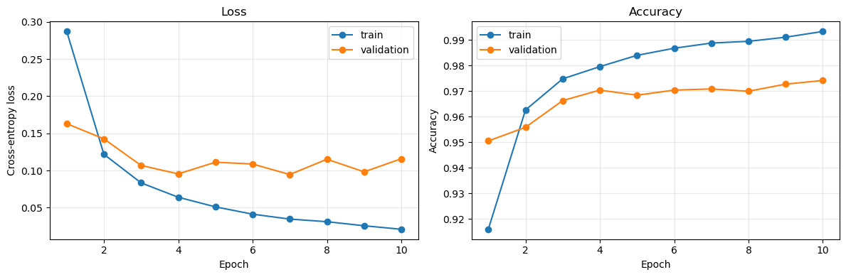
Epoch  1/10 | train loss 0.2870, acc 0.9160 | val loss 0.1630, acc 0.9506
Epoch  2/10 | train loss 0.1218, acc 0.9627 | val loss 0.1426, acc 0.9559
Epoch  3/10 | train loss 0.0834, acc 0.9748 | val loss 0.1068, acc 0.9663
Epoch  4/10 | train loss 0.0640, acc 0.9796 | val loss 0.0954, acc 0.9704
Epoch  5/10 | train loss 0.0511, acc 0.9840 | val loss 0.1112, acc 0.9684
Epoch  6/10 | train loss 0.0413, acc 0.9868 | val loss 0.1087, acc 0.9704
Epoch  7/10 | train loss 0.0347, acc 0.9888 | val loss 0.0946, acc 0.9709
Epoch  8/10 | train loss 0.0312, acc 0.9895 | val loss 0.1152, acc 0.9700
Epoch  9/10 | train loss 0.0257, acc 0.9911 | val loss 0.0983, acc 0.9728
Epoch 10/10 | train loss 0.0210, acc 0.9934 | val loss 0.1158, acc 0.9742
Step 8 — Results
8a. Training curves
The single most useful diagnostic plot in deep learning. Read it like this:
Both losses falling, close together → healthy learning.
Train loss falling, val loss rising → overfitting: the model is memorizing the training set.
Both losses flat and high → underfitting (too small a model, or learning rate is off).
Test loss:     0.1066
Test accuracy: 97.57%   (9,757 / 10,000 correct)
8c. Confusion matrix
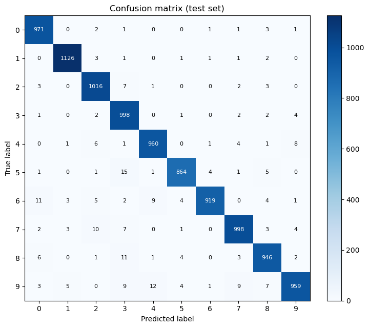
Accuracy is one number; the confusion matrix tells you which digits get confused with which. Row = true label, column = predicted label. A perfect model is purely diagonal.
First we collect all predictions on the test set.
@torch.no_grad()def get_predictions(model, loader): model.eval() all_preds, all_labels = [], []for X, y in loader: preds = model(X.to(device)).argmax(1).cpu() all_preds.append(preds) all_labels.append(y)return torch.cat(all_preds).numpy(), torch.cat(all_labels).numpy()y_pred, y_true = get_predictions(model, test_loader)# Build the 10x10 confusion matrix by hand -- it's just counting.cm = np.zeros((10, 10), dtype=int)for t, p inzip(y_true, y_pred): cm[t, p] +=1print("Confusion matrix shape:", cm.shape)
# Per-class accuracy = diagonal / row totalprint("Per-class accuracy:")for d inrange(10):print(f" digit {d}: {cm[d, d] / cm[d].sum() *100:5.2f}%")# Which off-diagonal mistakes are most common?mistakes = [(cm[i, j], i, j) for i inrange(10) for j inrange(10) if i != j]mistakes.sort(reverse=True)print("\nMost common confusions:")for n, i, j in mistakes[:5]:print(f" true {i} -> predicted {j}: {n} times")
Per-class accuracy:
  digit 0: 99.08%
  digit 1: 99.21%
  digit 2: 98.45%
  digit 3: 98.81%
  digit 4: 97.76%
  digit 5: 96.86%
  digit 6: 95.93%
  digit 7: 97.08%
  digit 8: 97.13%
  digit 9: 95.04%

Most common confusions:
  true 5 -> predicted 3: 15 times
  true 9 -> predicted 4: 12 times
  true 8 -> predicted 3: 11 times
  true 6 -> predicted 0: 11 times
  true 7 -> predicted 2: 10 times
8d. Error analysis — look at what it got wrong
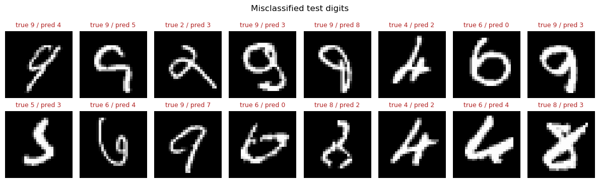
Numbers tell you that the model failed; the images tell you why. Many of these will be genuinely ambiguous digits that a human would also struggle with.
wrong_idx = np.where(y_pred != y_true)[0]print(f"{len(wrong_idx)} misclassified out of {len(y_true)}")fig, axes = plt.subplots(2, 8, figsize=(12, 3.8))for ax, idx inzip(axes.flat, wrong_idx[:16]): img, _ = test_set[idx] ax.imshow(unnormalize(img).squeeze(), cmap="gray") ax.set_title(f"true {y_true[idx]} / pred {y_pred[idx]}", fontsize=9, color="firebrick") ax.axis("off")plt.suptitle("Misclassified test digits")plt.tight_layout()plt.show()
243 misclassified out of 10000
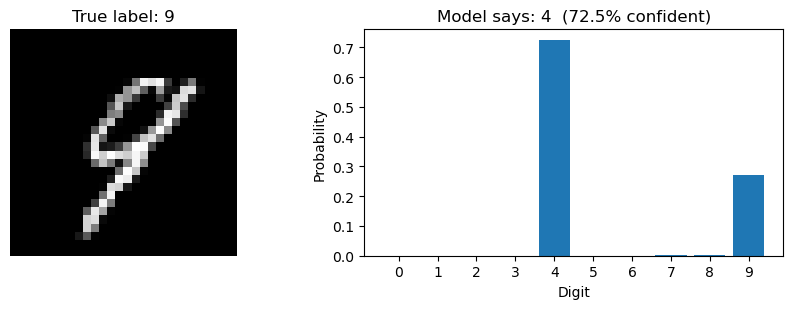
8e. Inspect the model’s confidence
The logits become probabilities via softmax. A well-behaved model is confident when it’s right, and often less confident when it’s wrong — which is useful information in the real world.
Standard practice: save the state_dict (the learned weights), not the whole Python object.
torch.save(model.state_dict(), "mnist_mlp.pth")# To reload later:# model = MLP().to(device)# model.load_state_dict(torch.load("mnist_mlp.pth"))# model.eval()print("Saved to mnist_mlp.pth")
Saved to mnist_mlp.pth
Recap
The workflow you just executed is the workflow, essentially unchanged, for image classifiers, text models, and everything in between:
Dataset — knows how to fetch sample i.
Explore — shapes, class balance, and look at the actual data.
Split — train / validation / test. Test is sacred; touch it once.
DataLoader — batching + shuffling.
nn.Module — __init__ defines the layers, forward defines the computation.
Loss + optimizer — what “wrong” means, and how to fix it.
The loop — zero_grad → forward → loss → backward → step.
Evaluate — curves, confusion matrix, error analysis. Not just one accuracy number.
Things to try
Set EPOCHS = 40. Does the validation loss eventually turn upward while training loss keeps falling? That’s overfitting, live.
Delete the two nn.ReLU() lines. Accuracy should collapse — you have built an (expensive) linear model.
Change lr=1e-3 to lr=1.0 and to lr=1e-6. Watch training break in two different ways.
Widen the hidden layer from 128 to 512. How much does accuracy improve per extra parameter?
Swap the MLP for a small CNN (nn.Conv2d). Everything else in this notebook stays exactly the same — that’s the payoff of a standard workflow.