Almost every deep learning project — no matter how fancy — follows the same seven steps:
#
Step
Question it answers
1
Load the data
What am I working with?
2
Explore & visualize
What does it actually look like?
3
Preprocess
What shape/scale does the network need?
4
Split train / validation
How will I know if I’m overfitting?
5
Build & compile the model
What function am I fitting, and how do I score it?
6
Train
Turn the crank.
7
Evaluate
Did it work? Where does it fail?
Our task: look at a 28×28 grayscale image of a handwritten digit and say which digit (0–9) it is.
Keep one idea in the back of your mind the whole time: a neural network is just a function. It takes 784 numbers in and produces 10 numbers out. Training is the process of nudging its internal knobs (weights) until that function is usually right.
0. Setup
import numpy as npimport matplotlib.pyplot as pltimport tensorflow as tffrom tensorflow import kerasfrom tensorflow.keras import layers# Fix the random seeds so the notebook is reproducible run-to-run.np.random.seed(42)tf.random.set_seed(42)print("TensorFlow:", tf.__version__)
TensorFlow: 2.13.0
1. Load the data
MNIST ships with Keras, so loading is a one-liner. It arrives already divided into a training set (60,000 images) and a test set (10,000 images).
The test set is a locked box. We will not look at it again until the very end.
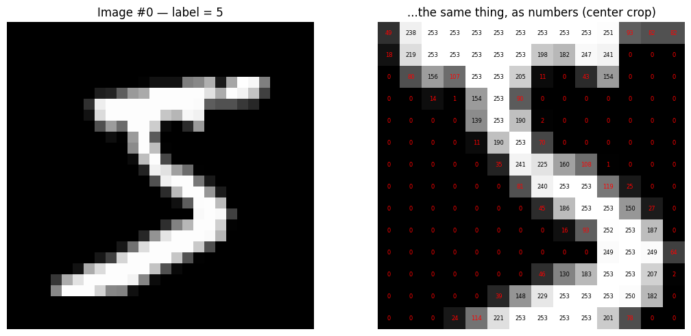
So each image is a 28 × 28 grid of integers from 0 to 255, where 0 = black (background) and 255 = white (ink).
That’s the key insight: an image is just a matrix of numbers. Let’s prove it by printing a corner of one.
img = x_train_full[0]label = y_train_full[0]fig, ax = plt.subplots(1, 2, figsize=(11, 5))# Left: the image as we see itax[0].imshow(img, cmap="gray")ax[0].set_title(f"Image #0 — label = {label}")ax[0].axis("off")# Right: the same image as the computer sees it (a 14x14 crop, values printed)crop = img[7:21, 7:21]ax[1].imshow(crop, cmap="gray")for i inrange(crop.shape[0]):for j inrange(crop.shape[1]): v = crop[i, j] ax[1].text(j, i, str(v), ha="center", va="center", fontsize=6, color="red"if v <128else"black")ax[1].set_title("...the same thing, as numbers (center crop)")ax[1].axis("off")plt.tight_layout()plt.show()
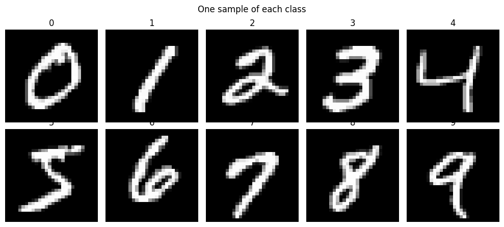
One example of each digit
fig, axes = plt.subplots(2, 5, figsize=(10, 4.5))for digit, ax inenumerate(axes.flat):# find the first image whose label is this digit idx = np.where(y_train_full == digit)[0][0] ax.imshow(x_train_full[idx], cmap="gray") ax.set_title(f"{digit}") ax.axis("off")plt.suptitle("One sample of each class")plt.tight_layout()plt.show()
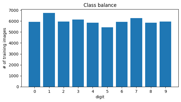
Are the classes balanced?
counts = np.bincount(y_train_full)plt.figure(figsize=(7, 3.5))plt.bar(range(10), counts)plt.xticks(range(10))plt.xlabel("digit")plt.ylabel("# of training images")plt.title("Class balance")plt.show()print(counts)
Roughly 6,000 images per digit — close enough to balanced that we don’t need to do anything special. (If one class had 50× fewer examples, accuracy would become a misleading metric and we’d have to be more careful.)
3. Preprocess
Two changes are needed to feed a plain MLP:
(a) Flatten. A dense layer takes a vector, not a grid. So we unroll each 28 × 28 image into a 784-long vector by reading it row by row.
Note what this throws away: the network no longer knows that pixel 5 and pixel 33 were vertical neighbors. An MLP has to rediscover spatial structure from scratch. This is exactly the weakness that convolutional networks fix — but it’s remarkable how far an MLP still gets.
(b) Rescale to [0, 1]. Divide by 255. Neural networks train much more stably when inputs are small and comparable in size; feeding in raw values up to 255 makes gradients large and erratic.
Training set → the model learns from this (weights are updated).
Validation set → the model never learns from this. We watch its score during training to detect overfitting and decide when to stop.
Test set → touched exactly once, at the end, for an honest final number.
If we tuned our choices by peeking at the test set, the test score would stop being an honest estimate of performance on new data. So we carve a validation set out of the training data.
from sklearn.model_selection import train_test_splitx_train, x_val, y_train, y_val = train_test_split( x_train_full_flat, y_train_full, test_size=0.2, # 20% held out for validation stratify=y_train_full, # keep the class balance in both halves random_state=42,)print("train:", x_train.shape[0], "images")print("val: ", x_val.shape[0], "images")print("test: ", x_test_flat.shape[0], "images")
Dense = “fully connected”: every neuron sees every value from the previous layer. Each neuron computes w · x + b — a weighted vote over its inputs.
relu = max(0, z). Without this nonlinearity, stacking layers would be pointless: a chain of linear maps collapses into a single linear map. ReLU is what lets the network build curved decision boundaries.
The layers get narrower (784 → 128 → 64 → 10). Think of it as a funnel: raw pixels → coarse strokes/edges → digit-ish features → a decision.
softmax on the last layer turns 10 arbitrary scores into 10 probabilities that sum to 1.
model = keras.Sequential([ layers.Input(shape=(784,)), layers.Dense(128, activation="relu"), layers.Dense(64, activation="relu"), layers.Dense(10, activation="softmax"),])model.summary()
Sanity-check the parameter count. Layer 1 has 784 × 128 weights plus 128 biases = 100,480 knobs. Layer 2: 128 × 64 + 64 = 8,256. Layer 3: 64 × 10 + 10 = 650. Total ≈ 109,386 numbers that training will adjust.
Compile = choose the scoring rule and the search strategy
compile() doesn’t train anything. It just attaches three things to the model:
loss — the number we are trying to make small. sparse_categorical_crossentropy is essentially “how surprised was the model by the correct answer?” It’s near 0 when the model puts high probability on the true digit, and blows up when it is confidently wrong. “Sparse” just means our labels are plain integers (7) rather than one-hot vectors ([0,...,1,...,0]).
optimizer — the rule for updating weights from the gradient. adam is the reliable default.
metrics — numbers we want reported but that aren’t used for the update. Accuracy is for humans; the loss is for the optimizer.
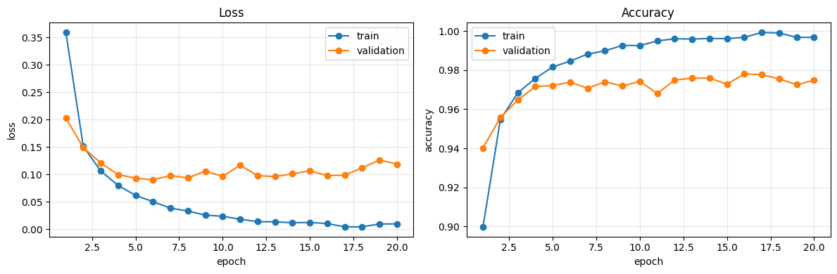
history.history is just a dictionary of lists — one value per epoch. Plotting it is the single most informative diagnostic in deep learning.
How to read these plots: - Both curves still falling → keep training. - Training loss falls, validation loss turns back up → overfitting: the model is memorizing training images instead of learning digits. - Both curves flat and high → underfitting (too small a model, or too few epochs).
Look at the gap between the two curves. The training accuracy climbs toward 100% while validation accuracy plateaus — that gap is overfitting, made visible. The model has enough capacity to start memorizing.
7b. Final evaluation on the test set
Now — and only now — we open the locked box.
test_loss, test_acc = model.evaluate(x_test_flat, y_test, verbose=0)print(f"Test loss: {test_loss:.4f}")print(f"Test accuracy: {test_acc:.4f} ({test_acc*100:.2f}%)")print(f"That's about {int(round((1-test_acc)*len(y_test)))} mistakes out of {len(y_test)} images.")
Test loss:     0.1084
Test accuracy: 0.9760   (97.60%)
That's about 240 mistakes out of 10000 images.
What the model actually outputs
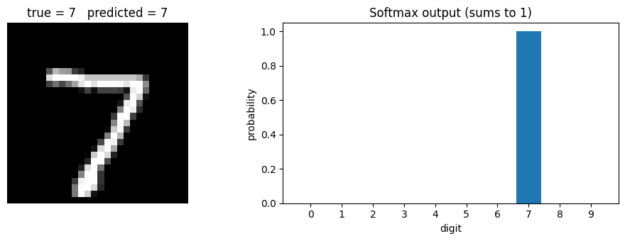
predict() returns 10 probabilities per image. To get a hard prediction we take the argmax — the index of the largest probability.
probs = model.predict(x_test_flat, verbose=0) # shape (10000, 10)y_pred = probs.argmax(axis=1) # shape (10000,)# Inspect a single test image and its full probability vectori =0fig, ax = plt.subplots(1, 2, figsize=(10, 3.5))ax[0].imshow(x_test[i], cmap="gray")ax[0].set_title(f"true = {y_test[i]} predicted = {y_pred[i]}")ax[0].axis("off")ax[1].bar(range(10), probs[i])ax[1].set_xticks(range(10))ax[1].set_xlabel("digit")ax[1].set_ylabel("probability")ax[1].set_title("Softmax output (sums to 1)")plt.tight_layout()plt.show()print("probabilities sum to:", probs[i].sum())
probabilities sum to: 0.9999999
7c. Confusion matrix
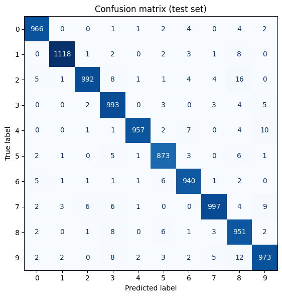
Accuracy is one number, and one number hides everything interesting. The confusion matrix tells us which digits get mistaken for which.
Row = the true digit. Column = what the model guessed. The diagonal is correct; everything off-diagonal is a mistake.
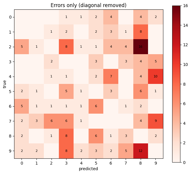
The diagonal dominates, so let’s zero it out and look only at the errors — that’s where the story is.
cm_errors = cm.copy()np.fill_diagonal(cm_errors, 0)fig, ax = plt.subplots(figsize=(7, 6))im = ax.imshow(cm_errors, cmap="Reds")ax.set_xticks(range(10)); ax.set_yticks(range(10))ax.set_xlabel("predicted"); ax.set_ylabel("true")ax.set_title("Errors only (diagonal removed)")for i inrange(10):for j inrange(10):if cm_errors[i, j] >0: ax.text(j, i, cm_errors[i, j], ha="center", va="center", fontsize=8)plt.colorbar(im)plt.tight_layout()plt.show()# The single worst confusion:i, j = np.unravel_index(cm_errors.argmax(), cm_errors.shape)print(f"Most common mistake: true {i} predicted as {j} ({cm_errors[i, j]} times)")
Most common mistake: true 2 predicted as 8 (16 times)
The mistakes are not random — they cluster where humans would also hesitate (4↔︎9, 3↔︎5, 7↔︎2). That’s reassuring: the model has learned something about shape, not noise.
Quick glossary for the columns: - precision — of everything the model called a 9, what fraction really was a 9? - recall — of all the actual 9s, what fraction did it catch? - f1-score — the harmonic mean of the two, a single balanced summary.
7d. Look at the failures
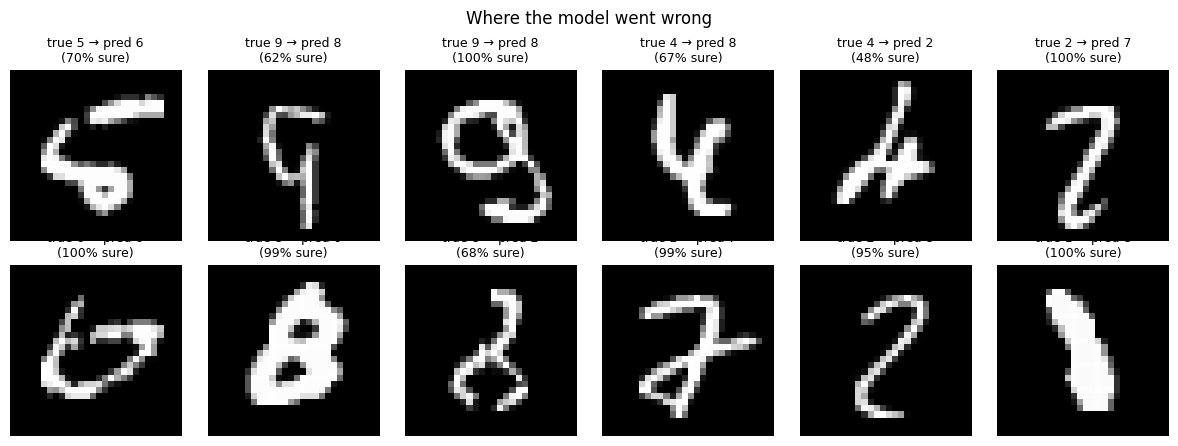
Always look at the images the model got wrong. It is the fastest way to build intuition about what the model is (and isn’t) doing.
wrong = np.where(y_pred != y_test)[0]print(f"{len(wrong)} misclassified test images")fig, axes = plt.subplots(2, 6, figsize=(12, 4.5))for ax, idx inzip(axes.flat, wrong[:12]): ax.imshow(x_test[idx], cmap="gray") confidence = probs[idx].max() ax.set_title(f"true {y_test[idx]} → pred {y_pred[idx]}\n({confidence:.0%} sure)", fontsize=9) ax.axis("off")plt.suptitle("Where the model went wrong")plt.tight_layout()plt.show()
240 misclassified test images
Many of these are genuinely ambiguous — sloppy handwriting that you might get wrong too. Notice also that the model is sometimes confidently wrong. A softmax probability is not a measure of how much the model actually knows.
Recap
You just executed the entire canonical workflow:
Load — keras.datasets.mnist.load_data()
Explore — shapes, ranges, class balance, sample images
Evaluate — training curves, test accuracy, confusion matrix, error inspection
This exact skeleton scales up. Swap MNIST for satellite images and the Dense stack for convolutions, and the seven steps do not change — only the contents of step 5.
Things to try
Remove the two hidden layers (leave only Dense(10, softmax)). You now have plain logistic regression — how much accuracy do you lose? That difference is what “deep” bought you.
Delete the activation="relu" arguments. Accuracy should collapse toward the linear model. Why?
Add layers.Dropout(0.2) after each hidden layer and re-look at the train/validation gap.
Skip the /255.0 rescaling and watch training struggle.
Train for 100 epochs and watch the validation loss curve turn upward — overfitting in the wild.